rm (list= ls ())library (sf)
Warning: Paket 'sf' wurde unter R Version 4.3.3 erstellt
Linking to GEOS 3.11.2, GDAL 3.8.2, PROJ 9.3.1; sf_use_s2() is TRUE
Warning: Paket 'terra' wurde unter R Version 4.3.3 erstellt
Warning: Paket 'ggplot2' wurde unter R Version 4.3.3 erstellt
Warning: Paket 'rprojroot' wurde unter R Version 4.3.3 erstellt
Warning: Paket 'patchwork' wurde unter R Version 4.3.3 erstellt
Attache Paket: 'patchwork'
Das folgende Objekt ist maskiert 'package:terra':

    area
= paste0 (find_rstudio_root_file (),"/tdv_session/data/" )
Introduction
In this tutorial we will explore the principles of design-based sampling. The simulation part is based on a presentation of Gerad Heuveling from Wageningen University, which he gave in the OpenGeoHub Summer School[https://opengeohub.org/summer-school/ogh-summer-school-2021/].
Learn how to draw a spatial random sample
Learn how to draw a systematic grid for a given area of interest
Run a simulation for design-based sampling
Data sets
For demonstration purposes we will work with a map of forest above ground biomass (AGB) produced by the Joint Research Center(JRC) for the European Union European Commission (Joint Research Centre (JRC) (2020) http://data.europa.eu/89h/d1fdf7aa-df33-49af-b7d5-40d226ec0da3.)
To provide a synthetic example we will assume that this map (agb_pop) is an error free representation of the population. Additionally we use a second map (agb_model) compiled using a machine learning model (RF) also depicting the AGB distribution.
= st_transform (st_read (paste0 (wd,"nlp-harz_aussengrenze.gpkg" )),25832 )
Reading layer `nlp-harz_aussengrenze' from data source
  `C:\Users\pmagdon\Documents\EON2024\tdv_session\data\nlp-harz_aussengrenze.gpkg'
  using driver `GPKG'
Simple feature collection with 1 feature and 3 fields
Geometry type: MULTIPOLYGON
Dimension:     XY
Bounding box:  xmin: 591196.6 ymin: 5725081 xmax: 619212.6 ymax: 5751232
Projected CRS: WGS 84 / UTM zone 32N
<- terra:: rast (paste0 (wd,"agb_np_harz_truth.tif" ))<- terra:: rast (paste0 (wd,"agb_np_harz_model.tif" ))
If we assume the \(z(x_i)=\) agb.pop to be an exact representation of the population we can calculate the Root mean Square Error (RMSE) as the difference between the model predictions \(\hat{z(x_i)}\) and the population map with:
\[
RMSE = \sqrt{\frac{1}{N}\sum{(z(x_{})-\hat{z}(x_{i}))^2}}
\]
= as.numeric (sqrt (terra:: global ((agb_pop- agb_model)^ 2 ,fun= 'mean' ,na.rm= TRUE )))
By looking at the difference from the “true” AGB and the difference we get a true RMSE of 41.23 t/ha.
Collect a random sample
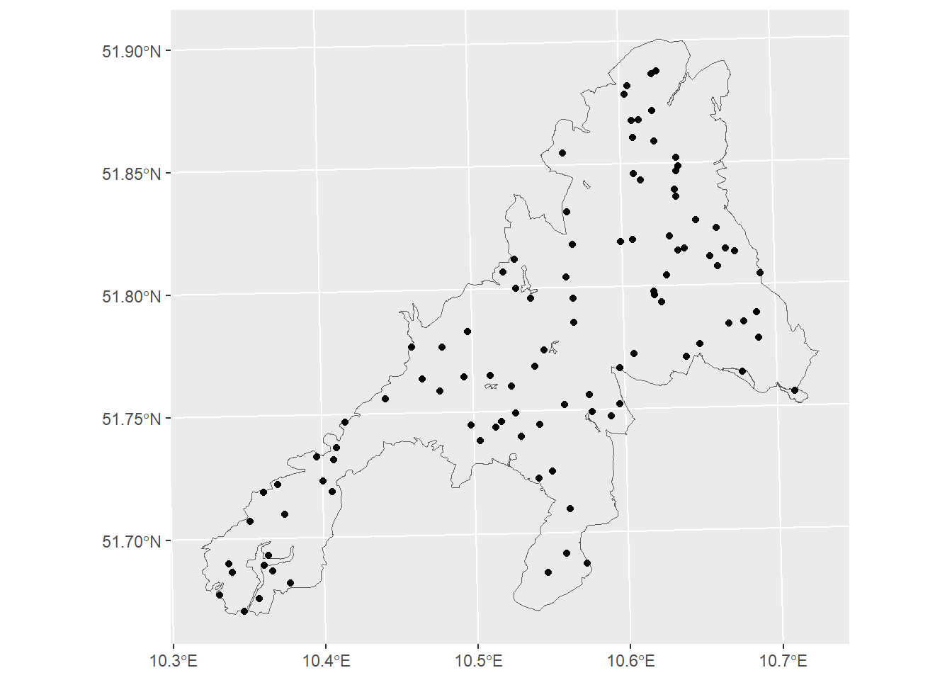
Since we know the true RMSE, we can test if a random sample estimate has a similar RMSE. We start with a random sample with \(n=100\) sample points.
= 100 = sf:: st_sample (np_boundary,size= n)ggplot ()+ geom_sf (data= np_boundary,fill= NA )+ geom_sf (data= p1)
We can now extract the population values and the model values at the sample locations and calculate the RMSE for all sample points.
<- terra:: extract ((agb_pop- agb_model),vect (p1))names (sample)<- c ('ID' ,'Diff' )<- sqrt (mean ((sample$ Diff)^ 2 ,na.rm= T))
The random sample estimates the RMSE as 41.05.
But is this an unbiased estimate?
Simulation of many random samples
To check if our sample based estimates are unbiased we will repeat the sampling \(k\) times.
<- agb_pop- agb_model<- 12324 names (dif)<- 'dif' <- 500 <- 50 <- rep (0 ,k) for (i in 1 : k) {print (i)= sf:: st_sample (np_boundary,size= n)<- terra:: extract (dif,vect (p1))<- sqrt (mean ((error$ dif)^ 2 ,na.rm= T))
[1] 1
[1] 2
[1] 3
[1] 4
[1] 5
[1] 6
[1] 7
[1] 8
[1] 9
[1] 10
[1] 11
[1] 12
[1] 13
[1] 14
[1] 15
[1] 16
[1] 17
[1] 18
[1] 19
[1] 20
[1] 21
[1] 22
[1] 23
[1] 24
[1] 25
[1] 26
[1] 27
[1] 28
[1] 29
[1] 30
[1] 31
[1] 32
[1] 33
[1] 34
[1] 35
[1] 36
[1] 37
[1] 38
[1] 39
[1] 40
[1] 41
[1] 42
[1] 43
[1] 44
[1] 45
[1] 46
[1] 47
[1] 48
[1] 49
[1] 50
[1] 51
[1] 52
[1] 53
[1] 54
[1] 55
[1] 56
[1] 57
[1] 58
[1] 59
[1] 60
[1] 61
[1] 62
[1] 63
[1] 64
[1] 65
[1] 66
[1] 67
[1] 68
[1] 69
[1] 70
[1] 71
[1] 72
[1] 73
[1] 74
[1] 75
[1] 76
[1] 77
[1] 78
[1] 79
[1] 80
[1] 81
[1] 82
[1] 83
[1] 84
[1] 85
[1] 86
[1] 87
[1] 88
[1] 89
[1] 90
[1] 91
[1] 92
[1] 93
[1] 94
[1] 95
[1] 96
[1] 97
[1] 98
[1] 99
[1] 100
[1] 101
[1] 102
[1] 103
[1] 104
[1] 105
[1] 106
[1] 107
[1] 108
[1] 109
[1] 110
[1] 111
[1] 112
[1] 113
[1] 114
[1] 115
[1] 116
[1] 117
[1] 118
[1] 119
[1] 120
[1] 121
[1] 122
[1] 123
[1] 124
[1] 125
[1] 126
[1] 127
[1] 128
[1] 129
[1] 130
[1] 131
[1] 132
[1] 133
[1] 134
[1] 135
[1] 136
[1] 137
[1] 138
[1] 139
[1] 140
[1] 141
[1] 142
[1] 143
[1] 144
[1] 145
[1] 146
[1] 147
[1] 148
[1] 149
[1] 150
[1] 151
[1] 152
[1] 153
[1] 154
[1] 155
[1] 156
[1] 157
[1] 158
[1] 159
[1] 160
[1] 161
[1] 162
[1] 163
[1] 164
[1] 165
[1] 166
[1] 167
[1] 168
[1] 169
[1] 170
[1] 171
[1] 172
[1] 173
[1] 174
[1] 175
[1] 176
[1] 177
[1] 178
[1] 179
[1] 180
[1] 181
[1] 182
[1] 183
[1] 184
[1] 185
[1] 186
[1] 187
[1] 188
[1] 189
[1] 190
[1] 191
[1] 192
[1] 193
[1] 194
[1] 195
[1] 196
[1] 197
[1] 198
[1] 199
[1] 200
[1] 201
[1] 202
[1] 203
[1] 204
[1] 205
[1] 206
[1] 207
[1] 208
[1] 209
[1] 210
[1] 211
[1] 212
[1] 213
[1] 214
[1] 215
[1] 216
[1] 217
[1] 218
[1] 219
[1] 220
[1] 221
[1] 222
[1] 223
[1] 224
[1] 225
[1] 226
[1] 227
[1] 228
[1] 229
[1] 230
[1] 231
[1] 232
[1] 233
[1] 234
[1] 235
[1] 236
[1] 237
[1] 238
[1] 239
[1] 240
[1] 241
[1] 242
[1] 243
[1] 244
[1] 245
[1] 246
[1] 247
[1] 248
[1] 249
[1] 250
[1] 251
[1] 252
[1] 253
[1] 254
[1] 255
[1] 256
[1] 257
[1] 258
[1] 259
[1] 260
[1] 261
[1] 262
[1] 263
[1] 264
[1] 265
[1] 266
[1] 267
[1] 268
[1] 269
[1] 270
[1] 271
[1] 272
[1] 273
[1] 274
[1] 275
[1] 276
[1] 277
[1] 278
[1] 279
[1] 280
[1] 281
[1] 282
[1] 283
[1] 284
[1] 285
[1] 286
[1] 287
[1] 288
[1] 289
[1] 290
[1] 291
[1] 292
[1] 293
[1] 294
[1] 295
[1] 296
[1] 297
[1] 298
[1] 299
[1] 300
[1] 301
[1] 302
[1] 303
[1] 304
[1] 305
[1] 306
[1] 307
[1] 308
[1] 309
[1] 310
[1] 311
[1] 312
[1] 313
[1] 314
[1] 315
[1] 316
[1] 317
[1] 318
[1] 319
[1] 320
[1] 321
[1] 322
[1] 323
[1] 324
[1] 325
[1] 326
[1] 327
[1] 328
[1] 329
[1] 330
[1] 331
[1] 332
[1] 333
[1] 334
[1] 335
[1] 336
[1] 337
[1] 338
[1] 339
[1] 340
[1] 341
[1] 342
[1] 343
[1] 344
[1] 345
[1] 346
[1] 347
[1] 348
[1] 349
[1] 350
[1] 351
[1] 352
[1] 353
[1] 354
[1] 355
[1] 356
[1] 357
[1] 358
[1] 359
[1] 360
[1] 361
[1] 362
[1] 363
[1] 364
[1] 365
[1] 366
[1] 367
[1] 368
[1] 369
[1] 370
[1] 371
[1] 372
[1] 373
[1] 374
[1] 375
[1] 376
[1] 377
[1] 378
[1] 379
[1] 380
[1] 381
[1] 382
[1] 383
[1] 384
[1] 385
[1] 386
[1] 387
[1] 388
[1] 389
[1] 390
[1] 391
[1] 392
[1] 393
[1] 394
[1] 395
[1] 396
[1] 397
[1] 398
[1] 399
[1] 400
[1] 401
[1] 402
[1] 403
[1] 404
[1] 405
[1] 406
[1] 407
[1] 408
[1] 409
[1] 410
[1] 411
[1] 412
[1] 413
[1] 414
[1] 415
[1] 416
[1] 417
[1] 418
[1] 419
[1] 420
[1] 421
[1] 422
[1] 423
[1] 424
[1] 425
[1] 426
[1] 427
[1] 428
[1] 429
[1] 430
[1] 431
[1] 432
[1] 433
[1] 434
[1] 435
[1] 436
[1] 437
[1] 438
[1] 439
[1] 440
[1] 441
[1] 442
[1] 443
[1] 444
[1] 445
[1] 446
[1] 447
[1] 448
[1] 449
[1] 450
[1] 451
[1] 452
[1] 453
[1] 454
[1] 455
[1] 456
[1] 457
[1] 458
[1] 459
[1] 460
[1] 461
[1] 462
[1] 463
[1] 464
[1] 465
[1] 466
[1] 467
[1] 468
[1] 469
[1] 470
[1] 471
[1] 472
[1] 473
[1] 474
[1] 475
[1] 476
[1] 477
[1] 478
[1] 479
[1] 480
[1] 481
[1] 482
[1] 483
[1] 484
[1] 485
[1] 486
[1] 487
[1] 488
[1] 489
[1] 490
[1] 491
[1] 492
[1] 493
[1] 494
[1] 495
[1] 496
[1] 497
[1] 498
[1] 499
[1] 500
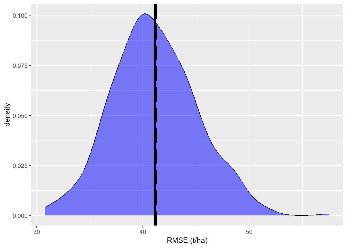
<- data.frame (x= RMSE, y= rep ('a' ,k))ggplot (data= df,aes (x= x))+ geom_density (data= subset (df,y== 'a' ),fill= 'blue' , alpha= 0.5 )+ xlab ('RMSE (t/ha)' )+ geom_vline (xintercept= RMSE_pop,linewidth= 1.5 ,color = 'black' , linetype= 'longdash' )+ geom_vline (xintercept= mean (df$ x),size= 1.5 ,color = 'black' )
Warning: Using `size` aesthetic for lines was deprecated in ggplot2 3.4.0.
ℹ Please use `linewidth` instead.
We see that the true RMSE and the mean of the \(k\) simulation runs are almost equal. Thus, we can assume an unbiased estimate of the RMSE.
But how does the sample size \(n\) affects the accuracy?
<- 500 <- 100 <- rep (0 ,k) for (i in 1 : k) {print (i)= sf:: st_sample (np_boundary,size= n)<- terra:: extract (dif,vect (p1))<- sqrt (mean ((error$ dif)^ 2 ,na.rm= T))
[1] 1
[1] 2
[1] 3
[1] 4
[1] 5
[1] 6
[1] 7
[1] 8
[1] 9
[1] 10
[1] 11
[1] 12
[1] 13
[1] 14
[1] 15
[1] 16
[1] 17
[1] 18
[1] 19
[1] 20
[1] 21
[1] 22
[1] 23
[1] 24
[1] 25
[1] 26
[1] 27
[1] 28
[1] 29
[1] 30
[1] 31
[1] 32
[1] 33
[1] 34
[1] 35
[1] 36
[1] 37
[1] 38
[1] 39
[1] 40
[1] 41
[1] 42
[1] 43
[1] 44
[1] 45
[1] 46
[1] 47
[1] 48
[1] 49
[1] 50
[1] 51
[1] 52
[1] 53
[1] 54
[1] 55
[1] 56
[1] 57
[1] 58
[1] 59
[1] 60
[1] 61
[1] 62
[1] 63
[1] 64
[1] 65
[1] 66
[1] 67
[1] 68
[1] 69
[1] 70
[1] 71
[1] 72
[1] 73
[1] 74
[1] 75
[1] 76
[1] 77
[1] 78
[1] 79
[1] 80
[1] 81
[1] 82
[1] 83
[1] 84
[1] 85
[1] 86
[1] 87
[1] 88
[1] 89
[1] 90
[1] 91
[1] 92
[1] 93
[1] 94
[1] 95
[1] 96
[1] 97
[1] 98
[1] 99
[1] 100
[1] 101
[1] 102
[1] 103
[1] 104
[1] 105
[1] 106
[1] 107
[1] 108
[1] 109
[1] 110
[1] 111
[1] 112
[1] 113
[1] 114
[1] 115
[1] 116
[1] 117
[1] 118
[1] 119
[1] 120
[1] 121
[1] 122
[1] 123
[1] 124
[1] 125
[1] 126
[1] 127
[1] 128
[1] 129
[1] 130
[1] 131
[1] 132
[1] 133
[1] 134
[1] 135
[1] 136
[1] 137
[1] 138
[1] 139
[1] 140
[1] 141
[1] 142
[1] 143
[1] 144
[1] 145
[1] 146
[1] 147
[1] 148
[1] 149
[1] 150
[1] 151
[1] 152
[1] 153
[1] 154
[1] 155
[1] 156
[1] 157
[1] 158
[1] 159
[1] 160
[1] 161
[1] 162
[1] 163
[1] 164
[1] 165
[1] 166
[1] 167
[1] 168
[1] 169
[1] 170
[1] 171
[1] 172
[1] 173
[1] 174
[1] 175
[1] 176
[1] 177
[1] 178
[1] 179
[1] 180
[1] 181
[1] 182
[1] 183
[1] 184
[1] 185
[1] 186
[1] 187
[1] 188
[1] 189
[1] 190
[1] 191
[1] 192
[1] 193
[1] 194
[1] 195
[1] 196
[1] 197
[1] 198
[1] 199
[1] 200
[1] 201
[1] 202
[1] 203
[1] 204
[1] 205
[1] 206
[1] 207
[1] 208
[1] 209
[1] 210
[1] 211
[1] 212
[1] 213
[1] 214
[1] 215
[1] 216
[1] 217
[1] 218
[1] 219
[1] 220
[1] 221
[1] 222
[1] 223
[1] 224
[1] 225
[1] 226
[1] 227
[1] 228
[1] 229
[1] 230
[1] 231
[1] 232
[1] 233
[1] 234
[1] 235
[1] 236
[1] 237
[1] 238
[1] 239
[1] 240
[1] 241
[1] 242
[1] 243
[1] 244
[1] 245
[1] 246
[1] 247
[1] 248
[1] 249
[1] 250
[1] 251
[1] 252
[1] 253
[1] 254
[1] 255
[1] 256
[1] 257
[1] 258
[1] 259
[1] 260
[1] 261
[1] 262
[1] 263
[1] 264
[1] 265
[1] 266
[1] 267
[1] 268
[1] 269
[1] 270
[1] 271
[1] 272
[1] 273
[1] 274
[1] 275
[1] 276
[1] 277
[1] 278
[1] 279
[1] 280
[1] 281
[1] 282
[1] 283
[1] 284
[1] 285
[1] 286
[1] 287
[1] 288
[1] 289
[1] 290
[1] 291
[1] 292
[1] 293
[1] 294
[1] 295
[1] 296
[1] 297
[1] 298
[1] 299
[1] 300
[1] 301
[1] 302
[1] 303
[1] 304
[1] 305
[1] 306
[1] 307
[1] 308
[1] 309
[1] 310
[1] 311
[1] 312
[1] 313
[1] 314
[1] 315
[1] 316
[1] 317
[1] 318
[1] 319
[1] 320
[1] 321
[1] 322
[1] 323
[1] 324
[1] 325
[1] 326
[1] 327
[1] 328
[1] 329
[1] 330
[1] 331
[1] 332
[1] 333
[1] 334
[1] 335
[1] 336
[1] 337
[1] 338
[1] 339
[1] 340
[1] 341
[1] 342
[1] 343
[1] 344
[1] 345
[1] 346
[1] 347
[1] 348
[1] 349
[1] 350
[1] 351
[1] 352
[1] 353
[1] 354
[1] 355
[1] 356
[1] 357
[1] 358
[1] 359
[1] 360
[1] 361
[1] 362
[1] 363
[1] 364
[1] 365
[1] 366
[1] 367
[1] 368
[1] 369
[1] 370
[1] 371
[1] 372
[1] 373
[1] 374
[1] 375
[1] 376
[1] 377
[1] 378
[1] 379
[1] 380
[1] 381
[1] 382
[1] 383
[1] 384
[1] 385
[1] 386
[1] 387
[1] 388
[1] 389
[1] 390
[1] 391
[1] 392
[1] 393
[1] 394
[1] 395
[1] 396
[1] 397
[1] 398
[1] 399
[1] 400
[1] 401
[1] 402
[1] 403
[1] 404
[1] 405
[1] 406
[1] 407
[1] 408
[1] 409
[1] 410
[1] 411
[1] 412
[1] 413
[1] 414
[1] 415
[1] 416
[1] 417
[1] 418
[1] 419
[1] 420
[1] 421
[1] 422
[1] 423
[1] 424
[1] 425
[1] 426
[1] 427
[1] 428
[1] 429
[1] 430
[1] 431
[1] 432
[1] 433
[1] 434
[1] 435
[1] 436
[1] 437
[1] 438
[1] 439
[1] 440
[1] 441
[1] 442
[1] 443
[1] 444
[1] 445
[1] 446
[1] 447
[1] 448
[1] 449
[1] 450
[1] 451
[1] 452
[1] 453
[1] 454
[1] 455
[1] 456
[1] 457
[1] 458
[1] 459
[1] 460
[1] 461
[1] 462
[1] 463
[1] 464
[1] 465
[1] 466
[1] 467
[1] 468
[1] 469
[1] 470
[1] 471
[1] 472
[1] 473
[1] 474
[1] 475
[1] 476
[1] 477
[1] 478
[1] 479
[1] 480
[1] 481
[1] 482
[1] 483
[1] 484
[1] 485
[1] 486
[1] 487
[1] 488
[1] 489
[1] 490
[1] 491
[1] 492
[1] 493
[1] 494
[1] 495
[1] 496
[1] 497
[1] 498
[1] 499
[1] 500
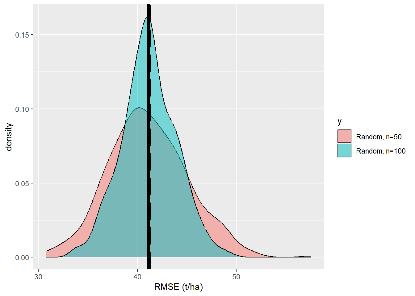
<- data.frame (x= RMSE_2, y= rep ('b' ,k))<- rbind (df,df_2)ggplot (data= df,aes (x= x,fill= y))+ geom_density (alpha= 0.5 )+ scale_fill_discrete (labels= c ('Random, n=50' , 'Random, n=100' ))+ xlab ('RMSE (t/ha)' )+ geom_vline (xintercept= RMSE_pop,size= 1.5 ,color = 'black' , linetype= 'longdash' )+ geom_vline (xintercept= mean (df$ x),size= 1.5 ,color = 'black' )
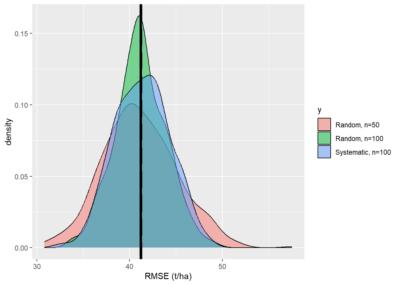
We see that the precision of the esimtates is increased. How much did the uncertainty decrease when we increase the sample size from \(n=50\) to \(n=100\) ?
Systematic sampling
Instead of a random sampling, systematic designs are more common in forest inventories for the following reasons:
Easy to establish and to document
Ensures a balanced spatial coverage
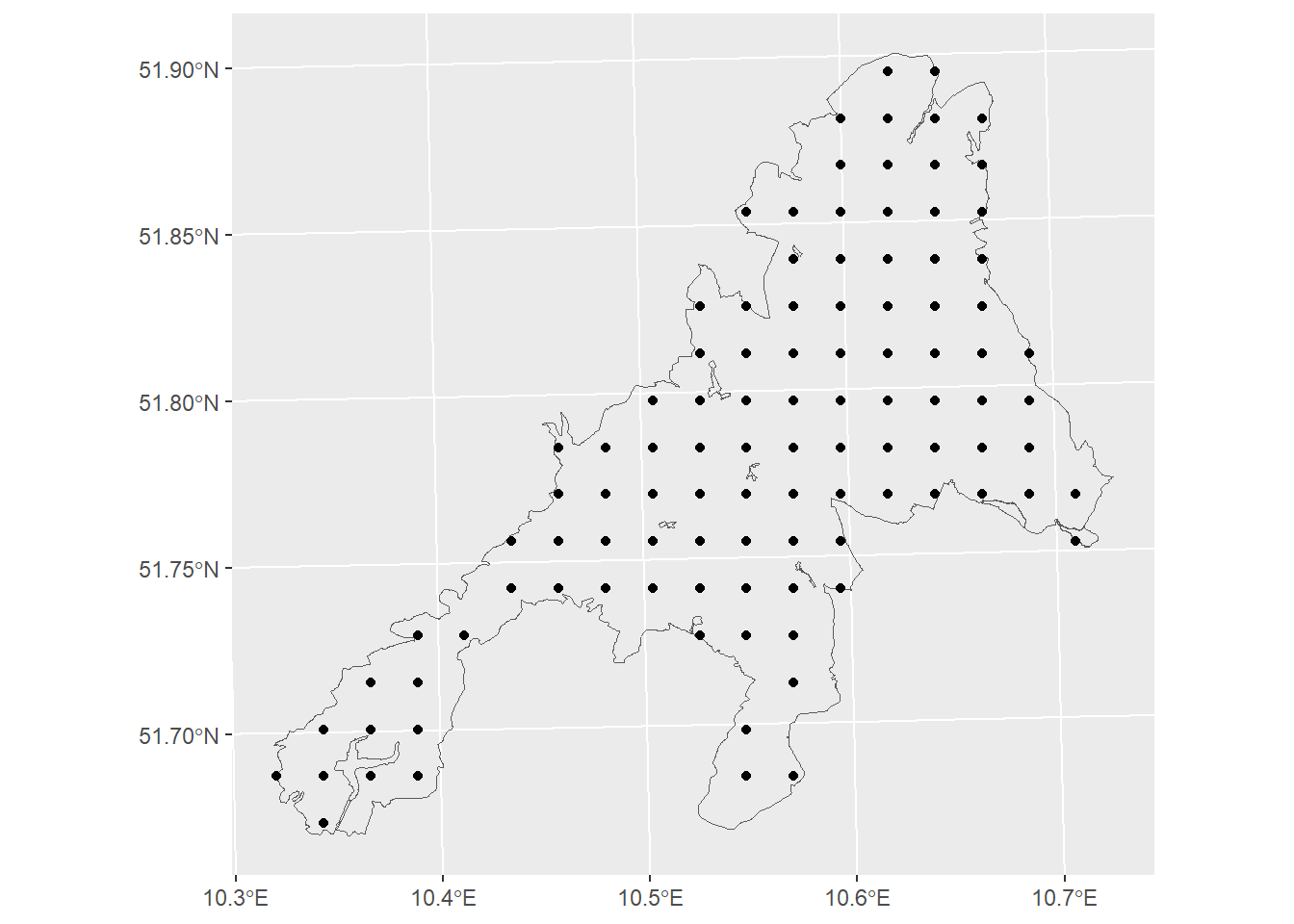
= sf:: st_sample (np_boundary,size= n,type= 'regular' )ggplot ()+ geom_sf (data= np_boundary,fill= NA )+ geom_sf (data= p1)
<- 500 <- 100 <- rep (0 ,k) for (i in 1 : k) {print (i)= sf:: st_sample (np_boundary,size= n,type= 'regular' )<- terra:: extract (dif,vect (p1))<- sqrt (mean ((error$ dif)^ 2 ,na.rm= T))
[1] 1
[1] 2
[1] 3
[1] 4
[1] 5
[1] 6
[1] 7
[1] 8
[1] 9
[1] 10
[1] 11
[1] 12
[1] 13
[1] 14
[1] 15
[1] 16
[1] 17
[1] 18
[1] 19
[1] 20
[1] 21
[1] 22
[1] 23
[1] 24
[1] 25
[1] 26
[1] 27
[1] 28
[1] 29
[1] 30
[1] 31
[1] 32
[1] 33
[1] 34
[1] 35
[1] 36
[1] 37
[1] 38
[1] 39
[1] 40
[1] 41
[1] 42
[1] 43
[1] 44
[1] 45
[1] 46
[1] 47
[1] 48
[1] 49
[1] 50
[1] 51
[1] 52
[1] 53
[1] 54
[1] 55
[1] 56
[1] 57
[1] 58
[1] 59
[1] 60
[1] 61
[1] 62
[1] 63
[1] 64
[1] 65
[1] 66
[1] 67
[1] 68
[1] 69
[1] 70
[1] 71
[1] 72
[1] 73
[1] 74
[1] 75
[1] 76
[1] 77
[1] 78
[1] 79
[1] 80
[1] 81
[1] 82
[1] 83
[1] 84
[1] 85
[1] 86
[1] 87
[1] 88
[1] 89
[1] 90
[1] 91
[1] 92
[1] 93
[1] 94
[1] 95
[1] 96
[1] 97
[1] 98
[1] 99
[1] 100
[1] 101
[1] 102
[1] 103
[1] 104
[1] 105
[1] 106
[1] 107
[1] 108
[1] 109
[1] 110
[1] 111
[1] 112
[1] 113
[1] 114
[1] 115
[1] 116
[1] 117
[1] 118
[1] 119
[1] 120
[1] 121
[1] 122
[1] 123
[1] 124
[1] 125
[1] 126
[1] 127
[1] 128
[1] 129
[1] 130
[1] 131
[1] 132
[1] 133
[1] 134
[1] 135
[1] 136
[1] 137
[1] 138
[1] 139
[1] 140
[1] 141
[1] 142
[1] 143
[1] 144
[1] 145
[1] 146
[1] 147
[1] 148
[1] 149
[1] 150
[1] 151
[1] 152
[1] 153
[1] 154
[1] 155
[1] 156
[1] 157
[1] 158
[1] 159
[1] 160
[1] 161
[1] 162
[1] 163
[1] 164
[1] 165
[1] 166
[1] 167
[1] 168
[1] 169
[1] 170
[1] 171
[1] 172
[1] 173
[1] 174
[1] 175
[1] 176
[1] 177
[1] 178
[1] 179
[1] 180
[1] 181
[1] 182
[1] 183
[1] 184
[1] 185
[1] 186
[1] 187
[1] 188
[1] 189
[1] 190
[1] 191
[1] 192
[1] 193
[1] 194
[1] 195
[1] 196
[1] 197
[1] 198
[1] 199
[1] 200
[1] 201
[1] 202
[1] 203
[1] 204
[1] 205
[1] 206
[1] 207
[1] 208
[1] 209
[1] 210
[1] 211
[1] 212
[1] 213
[1] 214
[1] 215
[1] 216
[1] 217
[1] 218
[1] 219
[1] 220
[1] 221
[1] 222
[1] 223
[1] 224
[1] 225
[1] 226
[1] 227
[1] 228
[1] 229
[1] 230
[1] 231
[1] 232
[1] 233
[1] 234
[1] 235
[1] 236
[1] 237
[1] 238
[1] 239
[1] 240
[1] 241
[1] 242
[1] 243
[1] 244
[1] 245
[1] 246
[1] 247
[1] 248
[1] 249
[1] 250
[1] 251
[1] 252
[1] 253
[1] 254
[1] 255
[1] 256
[1] 257
[1] 258
[1] 259
[1] 260
[1] 261
[1] 262
[1] 263
[1] 264
[1] 265
[1] 266
[1] 267
[1] 268
[1] 269
[1] 270
[1] 271
[1] 272
[1] 273
[1] 274
[1] 275
[1] 276
[1] 277
[1] 278
[1] 279
[1] 280
[1] 281
[1] 282
[1] 283
[1] 284
[1] 285
[1] 286
[1] 287
[1] 288
[1] 289
[1] 290
[1] 291
[1] 292
[1] 293
[1] 294
[1] 295
[1] 296
[1] 297
[1] 298
[1] 299
[1] 300
[1] 301
[1] 302
[1] 303
[1] 304
[1] 305
[1] 306
[1] 307
[1] 308
[1] 309
[1] 310
[1] 311
[1] 312
[1] 313
[1] 314
[1] 315
[1] 316
[1] 317
[1] 318
[1] 319
[1] 320
[1] 321
[1] 322
[1] 323
[1] 324
[1] 325
[1] 326
[1] 327
[1] 328
[1] 329
[1] 330
[1] 331
[1] 332
[1] 333
[1] 334
[1] 335
[1] 336
[1] 337
[1] 338
[1] 339
[1] 340
[1] 341
[1] 342
[1] 343
[1] 344
[1] 345
[1] 346
[1] 347
[1] 348
[1] 349
[1] 350
[1] 351
[1] 352
[1] 353
[1] 354
[1] 355
[1] 356
[1] 357
[1] 358
[1] 359
[1] 360
[1] 361
[1] 362
[1] 363
[1] 364
[1] 365
[1] 366
[1] 367
[1] 368
[1] 369
[1] 370
[1] 371
[1] 372
[1] 373
[1] 374
[1] 375
[1] 376
[1] 377
[1] 378
[1] 379
[1] 380
[1] 381
[1] 382
[1] 383
[1] 384
[1] 385
[1] 386
[1] 387
[1] 388
[1] 389
[1] 390
[1] 391
[1] 392
[1] 393
[1] 394
[1] 395
[1] 396
[1] 397
[1] 398
[1] 399
[1] 400
[1] 401
[1] 402
[1] 403
[1] 404
[1] 405
[1] 406
[1] 407
[1] 408
[1] 409
[1] 410
[1] 411
[1] 412
[1] 413
[1] 414
[1] 415
[1] 416
[1] 417
[1] 418
[1] 419
[1] 420
[1] 421
[1] 422
[1] 423
[1] 424
[1] 425
[1] 426
[1] 427
[1] 428
[1] 429
[1] 430
[1] 431
[1] 432
[1] 433
[1] 434
[1] 435
[1] 436
[1] 437
[1] 438
[1] 439
[1] 440
[1] 441
[1] 442
[1] 443
[1] 444
[1] 445
[1] 446
[1] 447
[1] 448
[1] 449
[1] 450
[1] 451
[1] 452
[1] 453
[1] 454
[1] 455
[1] 456
[1] 457
[1] 458
[1] 459
[1] 460
[1] 461
[1] 462
[1] 463
[1] 464
[1] 465
[1] 466
[1] 467
[1] 468
[1] 469
[1] 470
[1] 471
[1] 472
[1] 473
[1] 474
[1] 475
[1] 476
[1] 477
[1] 478
[1] 479
[1] 480
[1] 481
[1] 482
[1] 483
[1] 484
[1] 485
[1] 486
[1] 487
[1] 488
[1] 489
[1] 490
[1] 491
[1] 492
[1] 493
[1] 494
[1] 495
[1] 496
[1] 497
[1] 498
[1] 499
[1] 500
<- data.frame (x= RMSE_3, y= rep ('c' ,k))<- rbind (df,df_3)ggplot (data= df,aes (x= x, fill= y))+ geom_density (alpha= 0.5 )+ scale_fill_discrete (labels= c ('Random, n=50' , 'Random, n=100' ,'Systematic, n=100' ))+ xlab ('RMSE (t/ha)' )+ geom_vline (xintercept= RMSE_pop,size= 1.5 ,color = 'black' , linetype= 'longdash' )+ geom_vline (xintercept= mean (df$ x),size= 1.5 ,color = 'black' )
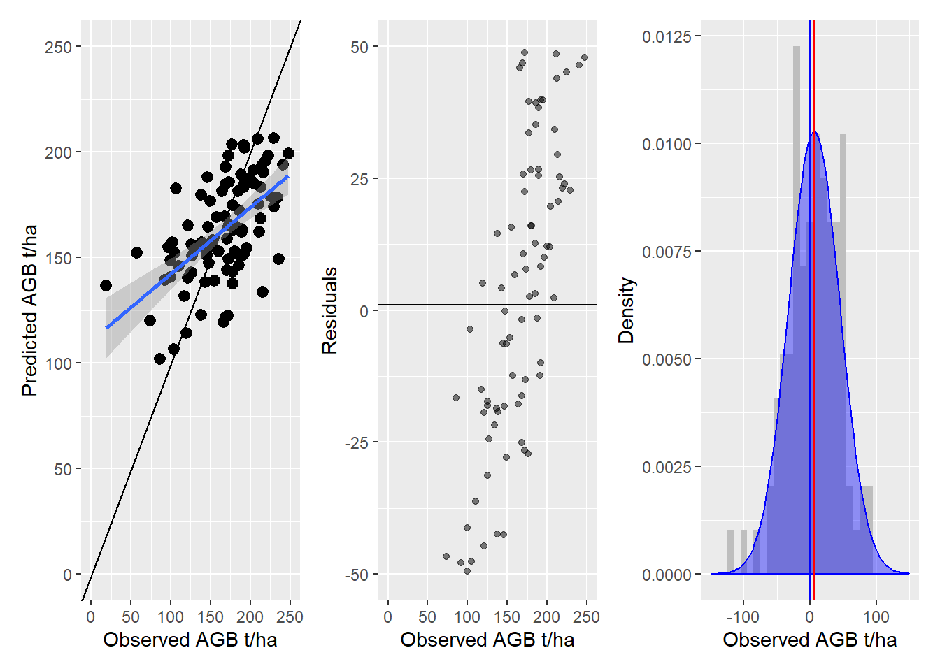
Evaluating the AGB-Model
Systematic sample to collect reference data for map validation
To validate the map we use a systematic sample grid. In a real world application we do not know the true population values. Therefore, field work would be needed to collect reference data at the selected sample points. In this workshop we assume that the agp_pop map represents the true value without any errors. Thus, we don’t need to go to field but we can sample the data by extracting the true values from the map at the sample locations.
# we will use n=100 sample plots = 100 = sf:: st_sample (np_boundary,size= n,type= 'regular' )ggplot ()+ geom_sf (data= np_boundary,fill= NA )+ geom_sf (data= p1)
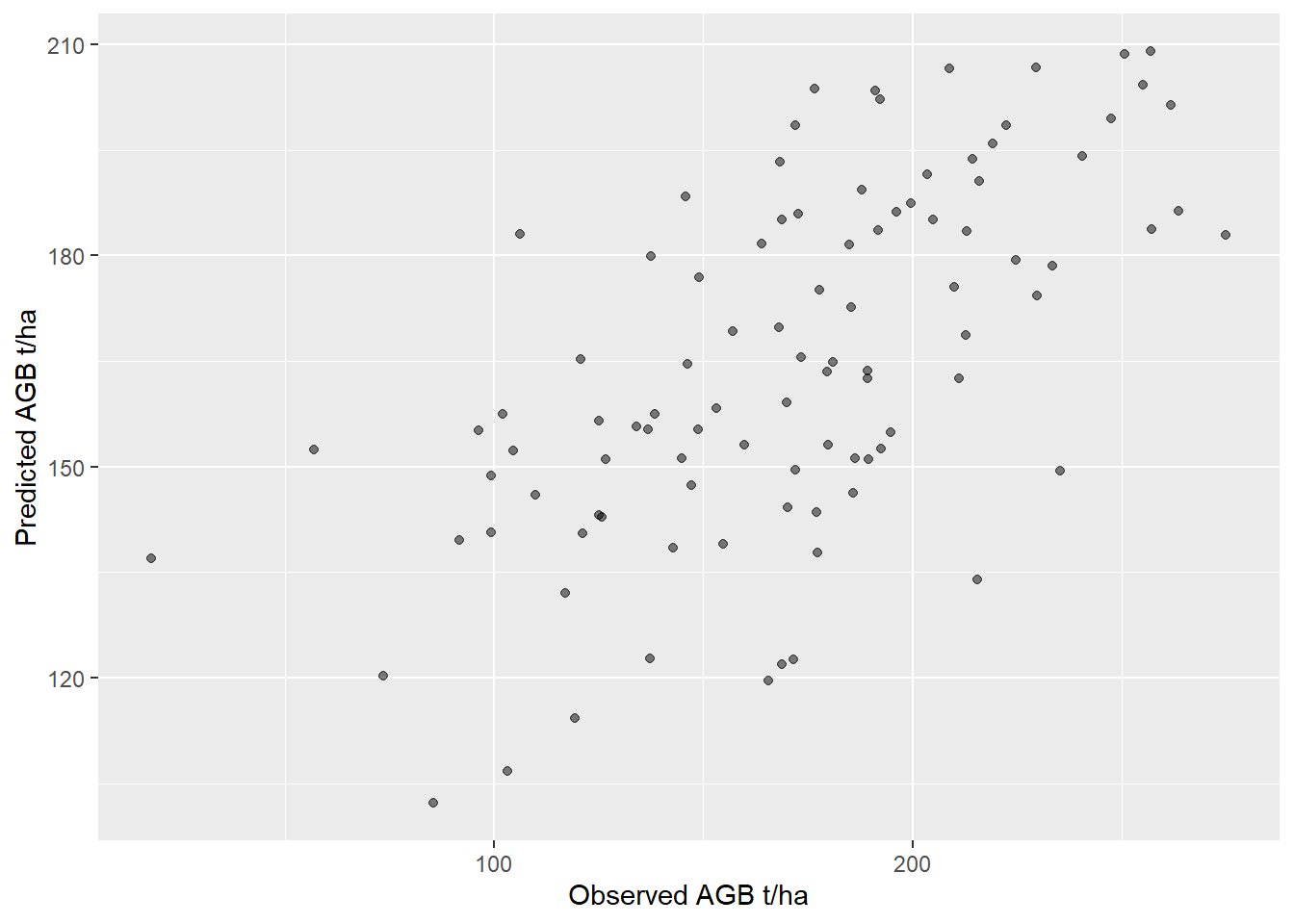
At each sample point we extract the predicted and observed AGB value.
<- terra:: extract (agb_pop,vect (p1))names (obs)<- c ('ID' ,'obs' )<- terra:: extract (agb_model,vect (p1))names (pred)<- c ('ID' ,'pred' )<- data.frame (observed= obs$ obs, predicted= pred$ pred)# we need to remove the na values from this dataframe. In real world applications # such NA values can, occur for example at inaccessible field plots. <- validation[complete.cases (validation),]