In this tutorial we will explore the principles of design-based sampling. The simulation part is based on a presentation of Gerad Heuveling from Wageningen University, which he gave in the OpenGeoHub Summer School[https://opengeohub.org/summer-school/ogh-summer-school-2021/].
Learn how to draw a spatial random sample
Learn how to draw a systematic grid for a given area of interest
Run a simulation for design-based sampling
Data sets
For demonstration purposes we will work with a map of forest above ground biomass (AGB) produced by the Joint Research Center(JRC) for the European Union European Commission (Joint Research Centre (JRC) (2020) http://data.europa.eu/89h/d1fdf7aa-df33-49af-b7d5-40d226ec0da3.)
To provide a synthetic example we will assume that this map (agb_pop) is an error free representation of the population. Additionally we use a second map (agb_model) compiled using a machine learning model (RF) also depicting the AGB distribution.
Before we can start you may download the following files:
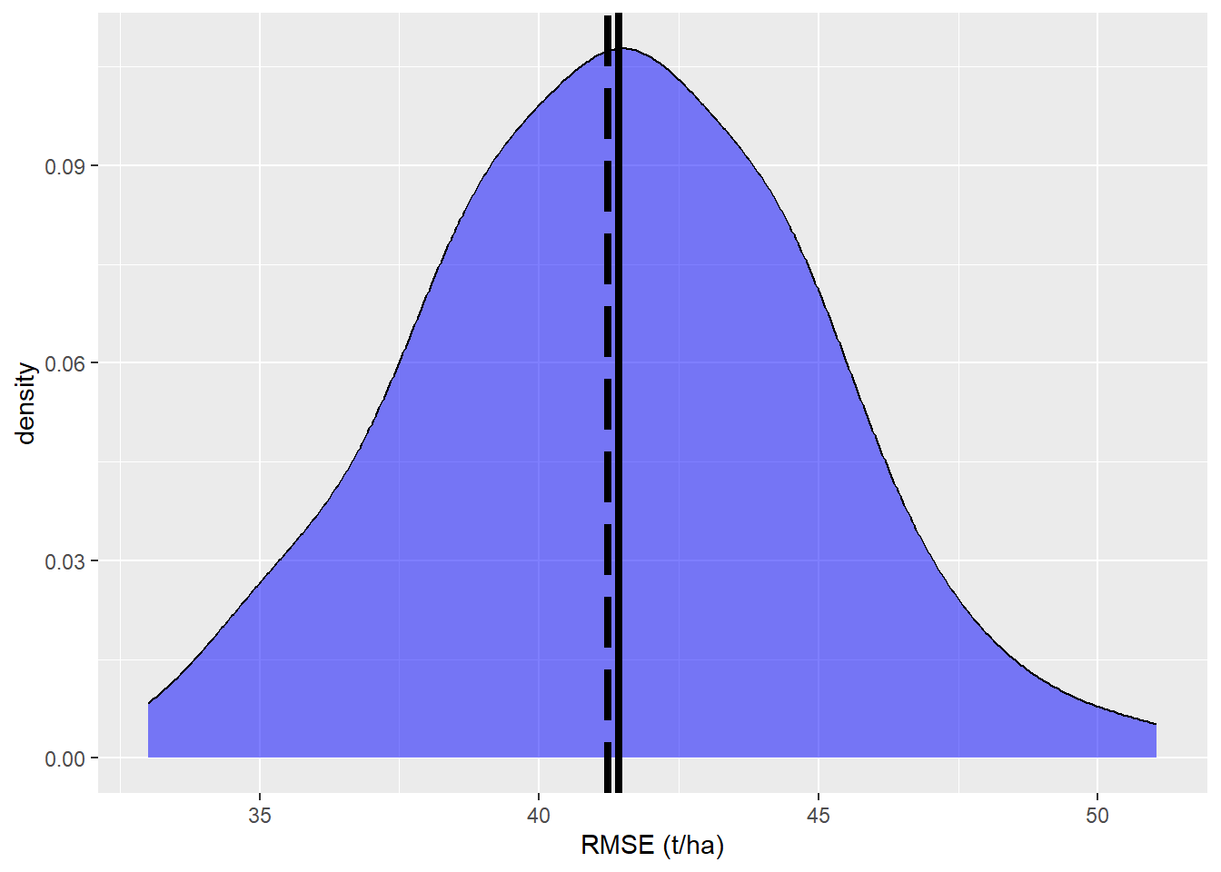
If we assume the \(z(x_i)=\) agb.pop to be an exact representation of the population we can calculate the Root mean Square Error (RMSE) as the difference between the model predictions \(\hat{z(x_i)}\) and the population map with:
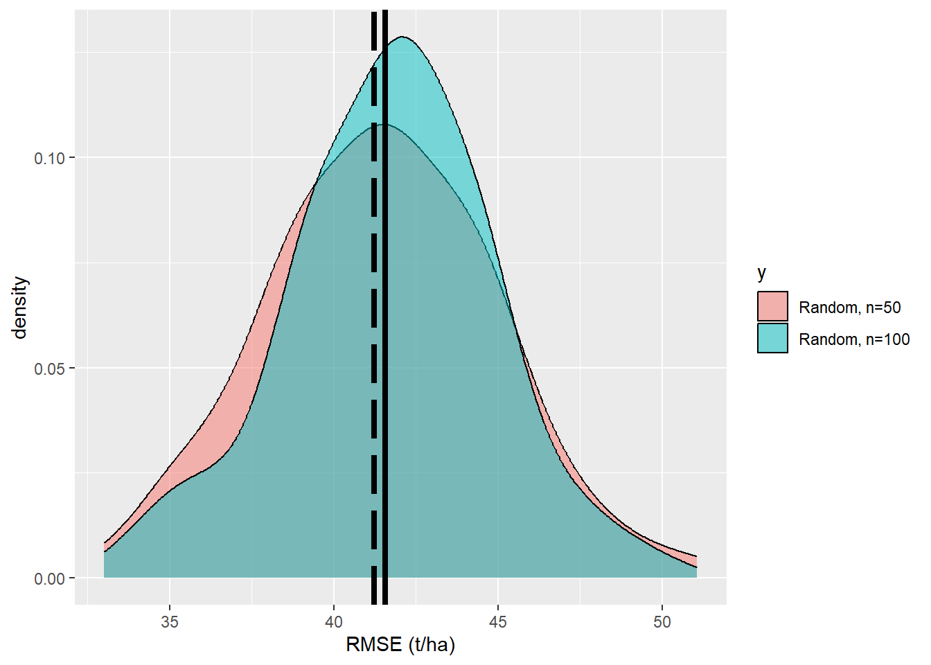
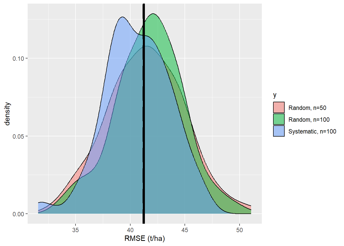
We see that the precision of the estimates is increased. How much did the uncertainty decrease when we increase the sample size from \(n=50\) to \(n=100\)?
sd(RMSE_2)/sd(RMSE)
[1] 0.8971176
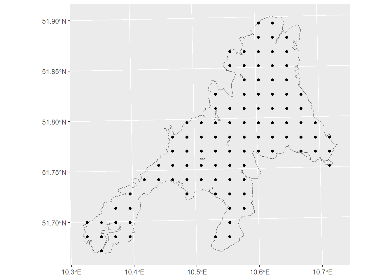
Systematic sampling
Instead of a random sampling, systematic designs are more common in forest inventories for the following reasons:
k <-100n <-100RMSE_3 <-rep(0,k) for (i in1:k) {print(i) p1 = sf::st_sample(np_boundary,size=n,type='regular') error<- terra::extract(dif,vect(p1)) RMSE_3[i] <-sqrt(mean((error$dif)^2,na.rm=T))}
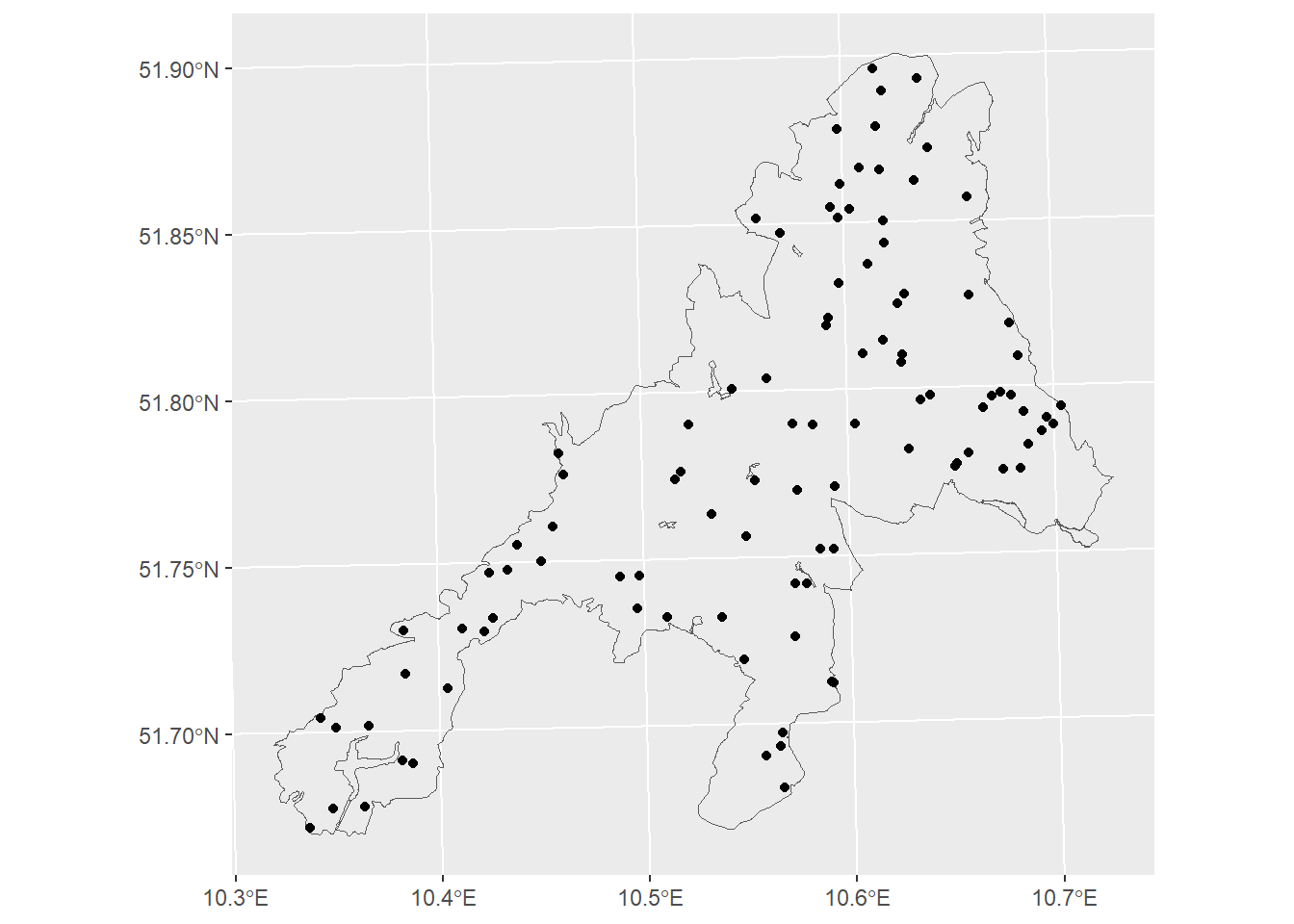
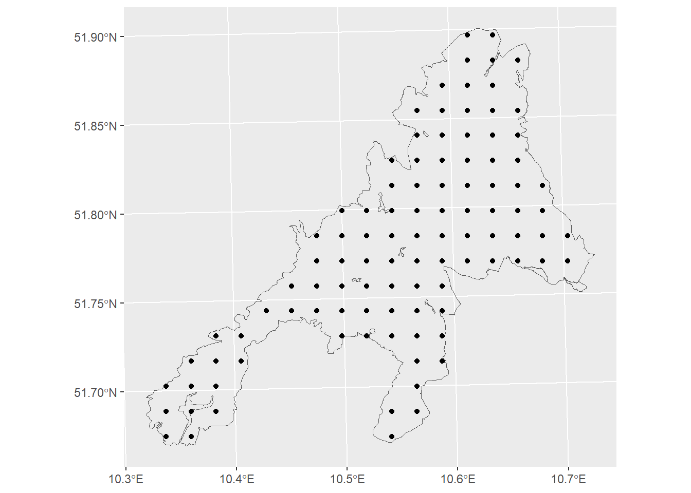
Systematic sample to collect reference data for map validation
To validate the map we use a systematic sample grid. In a real world application we do not know the true population values. Therefore, field work would be needed to collect reference data at the selected sample points. In this workshop we assume that the agp_pop map represents the true value without any errors. Thus, we don’t need to go to field but we can sample the data by extracting the true values from the map at the sample locations.
# we will use n=100 sample plotsn=100p1 = sf::st_sample(np_boundary,size=n,type='regular')ggplot()+geom_sf(data=np_boundary,fill=NA)+geom_sf(data=p1)
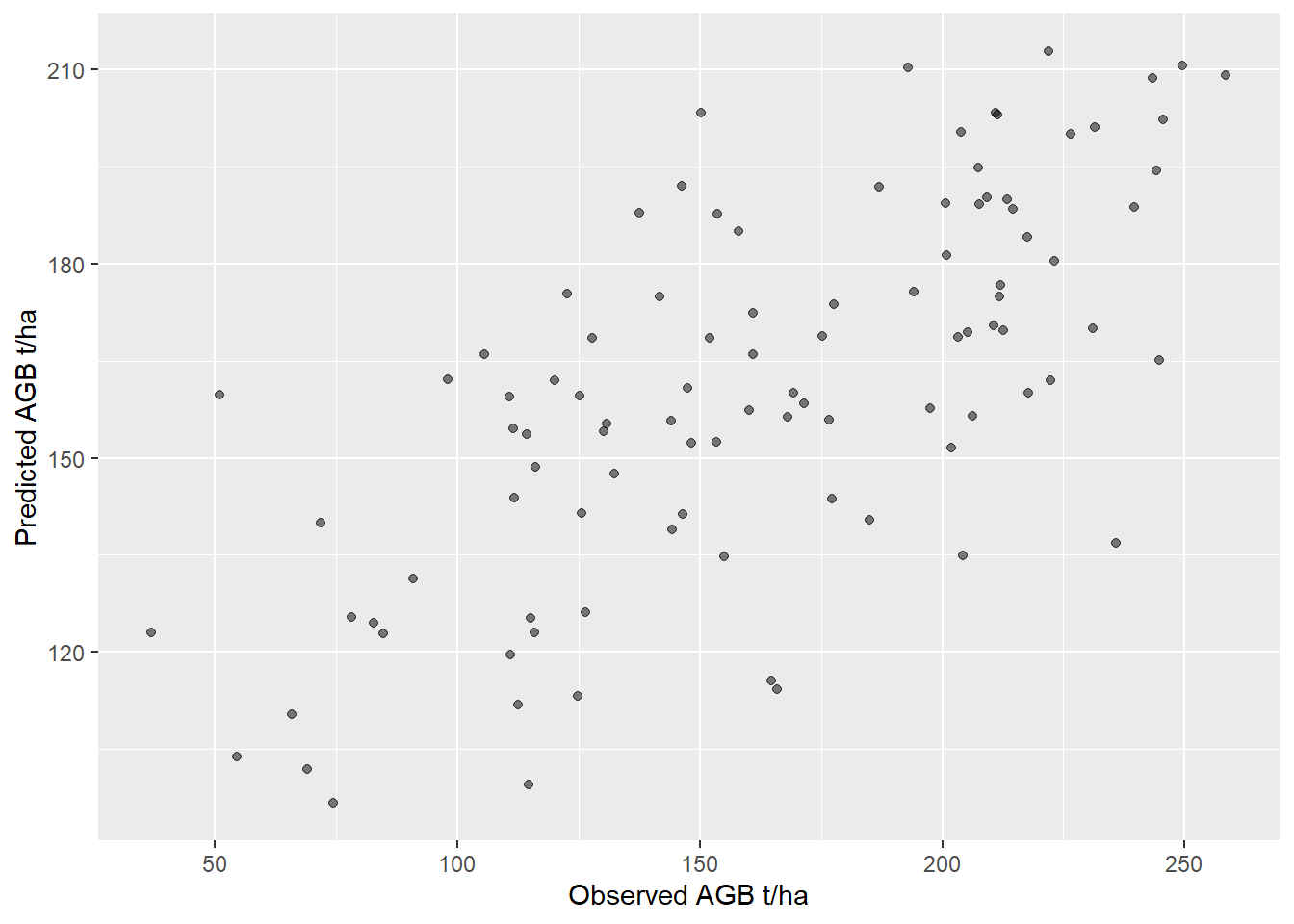
At each sample point we extract the predicted and observed AGB value.
obs <- terra::extract(agb_pop,vect(p1))names(obs)<-c('ID','obs')pred <- terra::extract(agb_model,vect(p1))names(pred)<-c('ID','pred')validation<-data.frame(observed=obs$obs, predicted=pred$pred)# we need to remove the na values from this dataframe. In real world applications# such NA values can, occur for example at inaccessible field plots.validation<-validation[complete.cases(validation),]
The sample RMSE is 38.89* t/ha. To better compare the values between different target variables and models is can also express as a proportion relative to the mean value of the predictions.
rRMSE = RMSE_sample/mean(validation$predicted)
On average we expect that the AGB estimate of our model has an error of 24.1 %.
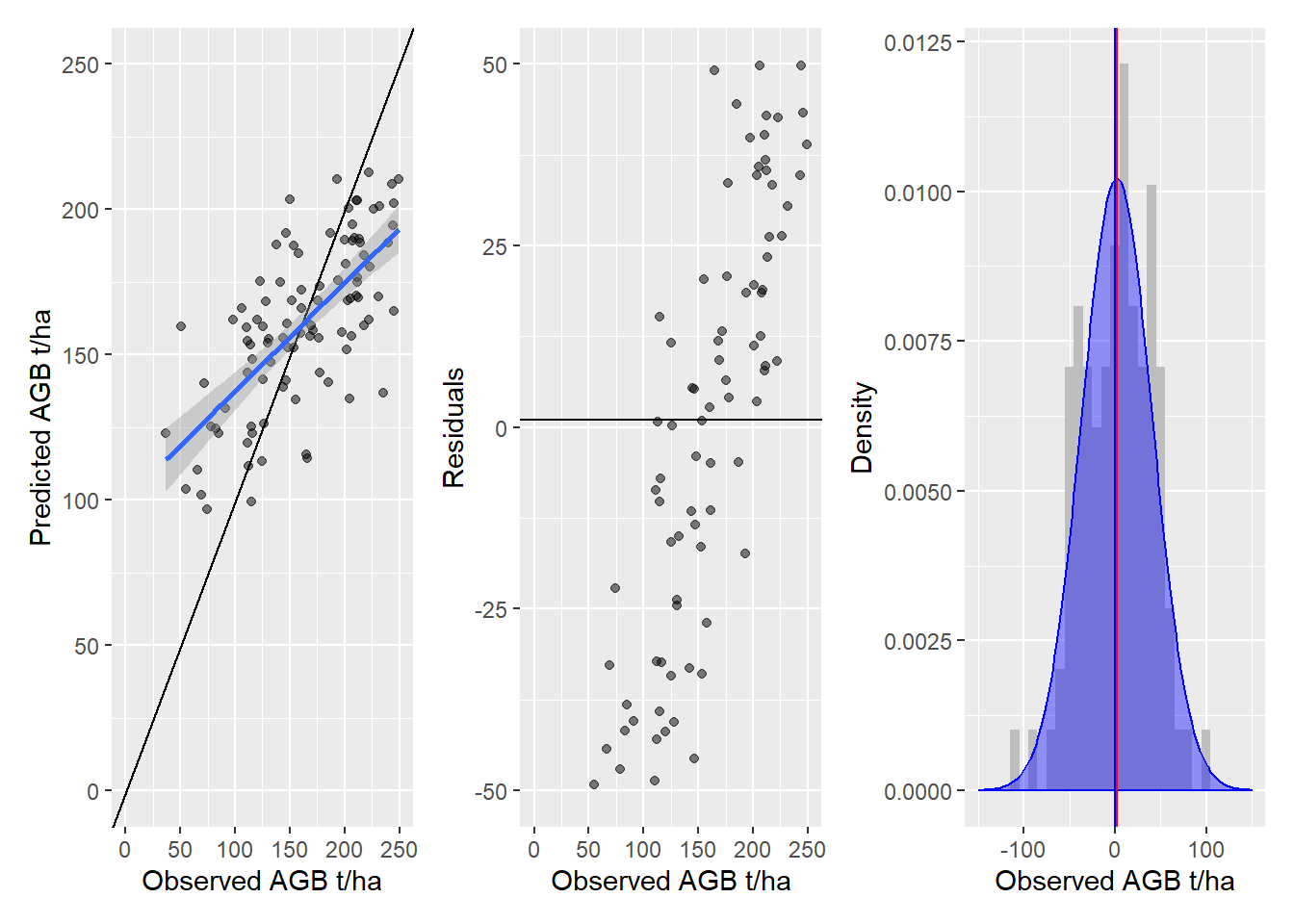
Error distribution
But is this RMSE valid for the entire range of the observed values or do we expect higher errors for higher AGB values?
To see how the model performs over target value range we can use the following analysis plots.