library(CAST)
library(terra)
library(caret)
library(randomForest)
library(mapview)
library(sf)
library(CAST)
library(tmap)Machine learning for remote sensing applications
Mapping the MarburgOpenForest
Slides and data
Slides and data are on https://github.com/earth-observation-network/EON2025/tree/main/ml_session
Introduction
In this tutorial we will go through the basic workflow of training machine learning models for spatial mapping based on remote sensing. To do this we will look at two case studies located in the MarburgOpenForest in Germany: one has the aim to produce a land cover map including different tree species; the other aims at producing a map of Leaf Area Index.
Based on “default” models, we will further discuss the relevance of different validation strategies and the area of applicability.
How to start
For this tutorial we need the terra package for processing of the satellite data as well as the caret package as a wrapper for machine learning (here: randomForest) algorithms. Sf is used for handling of the training data available as vector data (polygons). Mapview is used for spatial visualization of the data. CAST will be used to account for spatial dependencies during model validation as well as for the estimation of the AOA.
Case study 1: land cover classification
Data preparation
To start with, let’s load and explore the remote sensing raster data as well as the vector data that include the training sites.
Raster data (predictor variables)
mof_sen <- rast("data/sentinel_uniwald.grd")
print(mof_sen)
class : SpatRaster
dimensions : 522, 588, 10 (nrow, ncol, nlyr)
resolution : 10, 10 (x, y)
extent : 474200, 480080, 5629540, 5634760 (xmin, xmax, ymin, ymax)
coord. ref. : +proj=utm +zone=32 +datum=WGS84 +units=m +no_defs
source : sentinel_uniwald.grd
names : T32UM~1_B02, T32UM~1_B03, T32UM~1_B04, T32UM~1_B05, T32UM~1_B06, T32UM~1_B07, ...
min values : 723, 514, 294, 341.8125, 396.9375, 440.8125, ...
max values : 8325, 9087, 13810, 7368.7500, 8683.8125, 9602.3125, ... The raster data contain a subset of the optical data from Sentinel-2 (see band information here: https://en.wikipedia.org/wiki/Sentinel-2) given in scaled reflectances (B02-B11). In addition,the NDVI was calculated. Let’s plot the data to get an idea how the variables look like.
plot(mof_sen)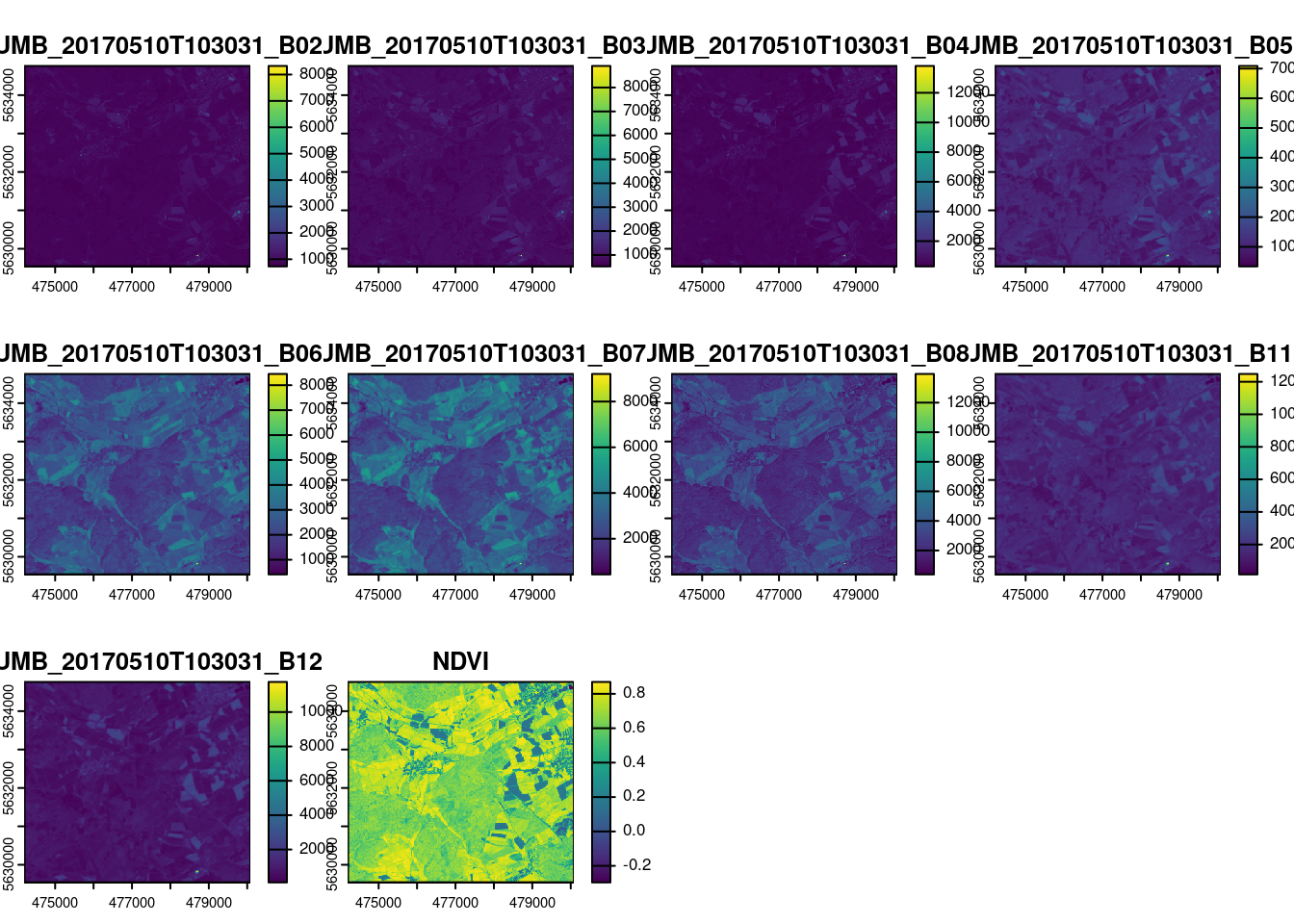
plotRGB(mof_sen,r=3,g=2,b=1,stretch="lin")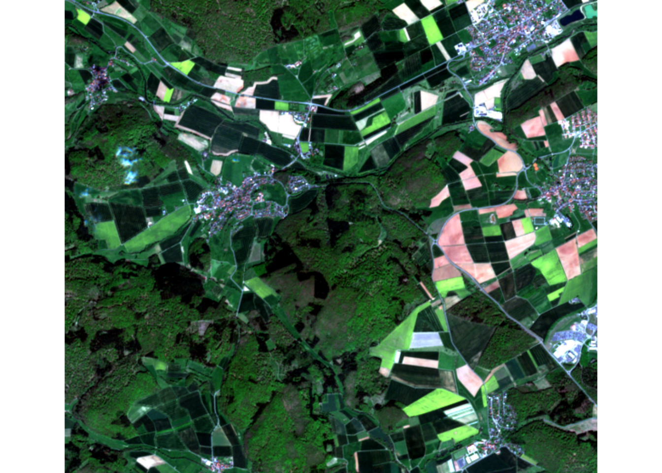
Vector data (Response variable)
The vector file is read as sf object. It contains the training sites that will be regarded here as a ground truth for the land cover classification.
trainSites <- read_sf("data/trainingsites_LUC.gpkg")Using mapview we can visualize the aerial image channels in the geographical context and overlay it with the polygons. Click on the polygons to see which land cover class is assigned to a respective polygon.
mapview(mof_sen[[1]], map.types = "Esri.WorldImagery") +
  mapview(trainSites)
Draw training samples and extract raster information
In order to train a machine learning model between the spectral properties and the land cover class, we first need to create a data frame that contains the predictor variables at the location of the training sites as well as the corresponding class information. However, using each pixel overlapped by a polygon would lead to a overly huge dataset, therefore, we first draw training samples from the polygon. Let’s use 1000 randomly sampled (within the polygons) pixels as training data set.
trainlocations <- st_sample(trainSites,1000)
trainlocations <- st_join(st_sf(trainlocations), trainSites)
mapview(trainlocations)
Next, we can extract the raster values for these locations. The resulting data frame contains the predictor variables for each training location that we can merged with the information on the land cover class from the sf object.
trainDat <- extract(mof_sen, trainlocations, df=TRUE)
trainDat <- data.frame(trainDat, trainlocations)
head(trainDat)
ID T32UMB_20170510T103031_B02 T32UMB_20170510T103031_B03
1 1 1243 1169
2 2 885 784
3 3 827 785
4 4 915 848
5 5 804 689
6 6 923 1054
T32UMB_20170510T103031_B04 T32UMB_20170510T103031_B05
1 926 1143.500
2 568 935.000
3 501 1077.750
4 731 1147.438
5 445 901.500
6 733 1260.812
T32UMB_20170510T103031_B06 T32UMB_20170510T103031_B07
1 2252.312 2552.812
2 2242.188 2766.938
3 2148.500 2483.250
4 1893.750 2129.688
5 1747.125 2002.500
6 3734.625 4639.625
T32UMB_20170510T103031_B08 T32UMB_20170510T103031_B11
1 2925 1878.812
2 2644 1523.062
3 2385 1359.500
4 2114 1788.312
5 1812 1183.062
6 4769 1205.312
T32UMB_20170510T103031_B12 NDVI id LN Type trainlocations
1 1303.5625 0.5190859 64 503 Wasser POINT (476609.7 5632431)
2 824.1250 0.6463263 NA 106 Felder POINT (478523.8 5631097)
3 635.2500 0.6528066 NA 2 Buche POINT (477490.4 5632300)
4 1003.6250 0.4861160 NA 2 Buche POINT (477605.7 5631966)
5 558.5625 0.6056712 NA 1 Eiche POINT (476782.9 5632857)
6 523.8125 0.7335514 NA 102 Felder POINT (478600.8 5631513)Model training
Predictors and response
For model training we need to define the predictor and response variables. As predictors we can use basically all information from the raster stack as we might assume they could all be meaningful for the differentiation between the land cover classes. As response variable we use the “Label” column of the data frame.
predictors <- names(mof_sen)
response <- "Type"
A first “default” model
We then train a Random Forest model to lean how the classes can be distinguished based on the predictors (note: other algorithms would work as well. See https://topepo.github.io/caret/available-models.html for a list of algorithms available in caret). Caret’s train function is doing this job.
So let’s see how we can then train a “default” random forest model. We specify “rf” as method, indicating that a Random Forest is applied. We reduce the number of trees (ntree) to 75 to speed things up. Note that usually a larger number (>250) is appropriate.
model <- train(trainDat[,predictors],
               trainDat[,response],
               method="rf",
               ntree=75)
model
Random Forest
1000 samples
10 predictor
10 classes: 'Buche', 'Duglasie', 'Eiche', 'Felder', 'Fichte', 'Laerche', 'Siedlung', 'Strasse', 'Wasser', 'Wiese'
No pre-processing
Resampling: Bootstrapped (25 reps)
Summary of sample sizes: 1000, 1000, 1000, 1000, 1000, 1000, ...
Resampling results across tuning parameters:
mtry Accuracy Kappa
2 0.8309292 0.7895740
6 0.8341677 0.7942385
10 0.8271947 0.7855348
Accuracy was used to select the optimal model using the largest value.
The final value used for the model was mtry = 6.To perform the classification we can then use the trained model and apply it to each pixel of the raster stack using the predict function.
prediction <- predict(mof_sen,model)Then we can then create a map with meaningful colors of the predicted land cover using the tmap package.
cols <- rev(c("palegreen", "blue", "grey", "red", "lightgreen", "forestgreen", "beige","brown","darkgreen","yellowgreen"))

tm_shape(prediction) +
  tm_raster(palette = cols,title = "LUC")+
  tm_scale_bar(bg.color="white",bg.alpha=0.75)+
  tm_layout(legend.bg.color = "white",
            legend.bg.alpha = 0.75)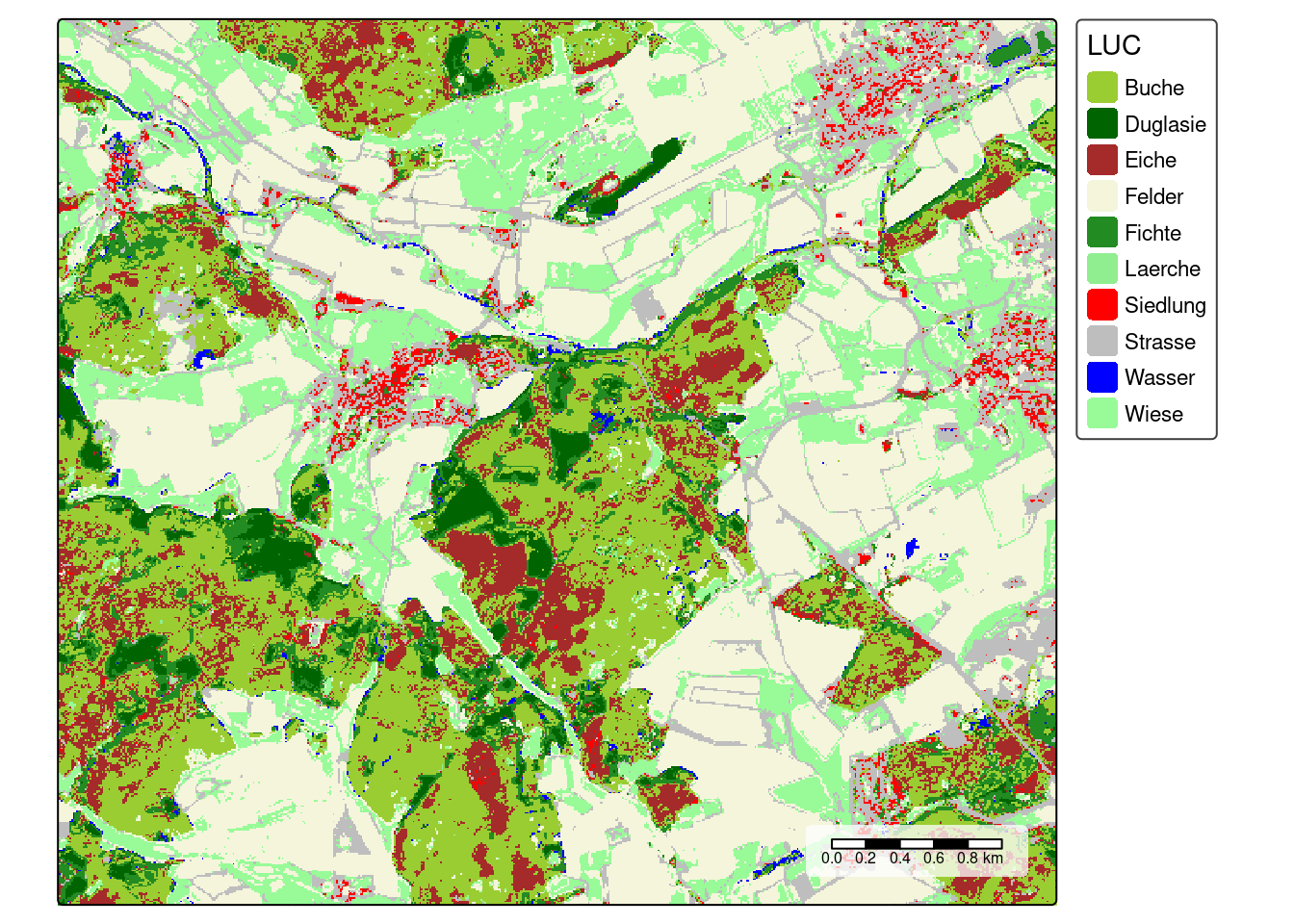
Based on this we can now discuss more advanced aspects of cross-validation for performance assessment as well as spatial variable selection strategies.
Model training with spatial CV and variable selection
Before starting model training we can specify some control settings using trainControl. For hyperparameter tuning (mtry) as well as for error assessment we use a spatial cross-validation. Here, the training data are split into 5 folds by trying to resemble the geographic distance distribution required when predicting the entire area from the trainign data,
indices <- knndm(trainlocations,mof_sen,k=5)
gd <- geodist(trainlocations,mof_sen,cvfolds = indices$indx_train)
plot(gd)+ scale_x_log10(labels=round)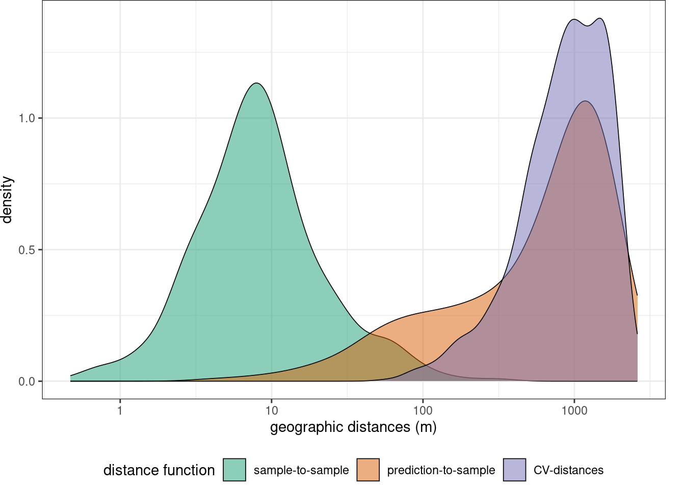
ctrl <- trainControl(method="cv",
                     index = indices$indx_train,
                     indexOut = indices$indx_test,
                     savePredictions = TRUE)
Model training is then again performed using caret’s train function. However we use a wrapper around it that is selecting the predictor variables which are relevant for making predictions to new spatial locations (forward feature selection, fss). We use the Kappa index as metric to select the best model.
# train the model
set.seed(100)
model <- ffs(trainDat[,predictors],
             trainDat[,response],
             method="rf",
             metric="Kappa",
             trControl=ctrl,
             importance=TRUE,
             ntree=100,
verbose=FALSE)print(model)Selected Variables:
T32UMB_20170510T103031_B05 T32UMB_20170510T103031_B06 T32UMB_20170510T103031_B02 T32UMB_20170510T103031_B11 T32UMB_20170510T103031_B12
---
Random Forest
1000 samples
5 predictor
10 classes: 'Buche', 'Duglasie', 'Eiche', 'Felder', 'Fichte', 'Laerche', 'Siedlung', 'Strasse', 'Wasser', 'Wiese'
No pre-processing
Resampling: Cross-Validated (10 fold)
Summary of sample sizes: 768, 791, 712, 854, 875
Resampling results across tuning parameters:
mtry Accuracy Kappa
2 0.7562707 0.5637556
3 0.7492029 0.5575426
5 0.7344652 0.5369017
Kappa was used to select the optimal model using the largest value.
The final value used for the model was mtry = 2.plot(varImp(model))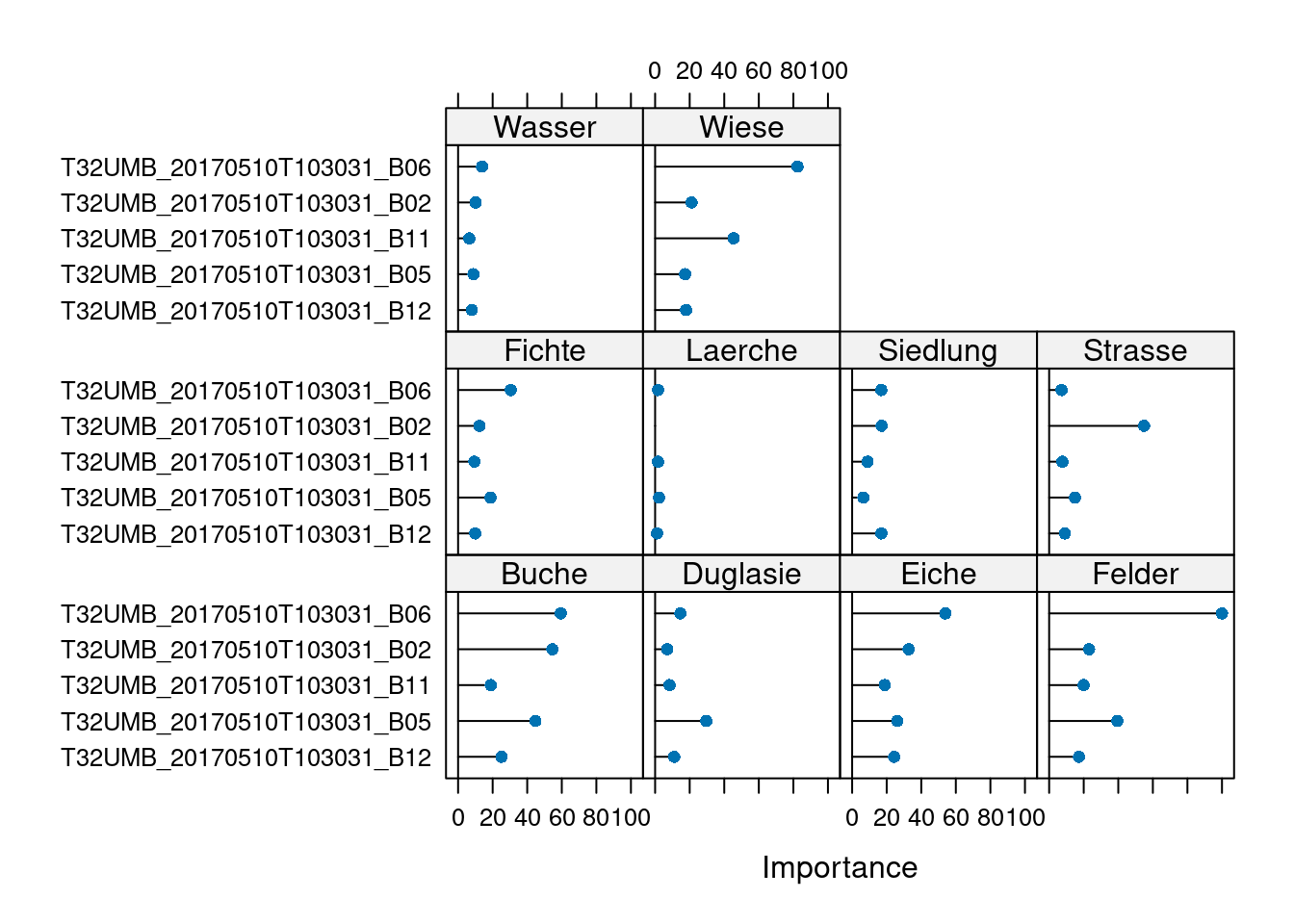
Model validation
When we print the model (see above) we get a summary of the prediction performance as the average Kappa and Accuracy of the three spatial folds. Looking at all cross-validated predictions together we can get the “global” model performance.
# get all cross-validated predictions:
cvPredictions <- model$pred[model$pred$mtry==model$bestTune$mtry,]
# calculate cross table:
table(cvPredictions$pred,cvPredictions$obs)
           Buche Duglasie Eiche Felder Fichte Laerche Siedlung Strasse Wasser
  Buche        4        0     2      2     11       0        0       0      0
  Duglasie     0        0     0      1      3       0        0       0      0
  Eiche        0        0     1      2      2       0        0       0      0
  Felder       6        0     0    259      0       0        0       6      0
  Fichte       0        0     0      3      0       0        0       0      0
  Laerche      0        0     0      0      0       0        0       0      0
  Siedlung     0        0     0      0      0       0        0       0      0
  Strasse      0        0     0     16      0       0        0      25      0
  Wasser       0        0     0      2      3       0        0       0      0
  Wiese        0        0     0     30      0       0        0       9      0

           Wiese
  Buche        0
  Duglasie     0
  Eiche        1
  Felder       6
  Fichte       0
  Laerche      0
  Siedlung     0
  Strasse      8
  Wasser       0
  Wiese       78
Visualize the final model predictions
prediction <- predict(mof_sen,model)
cols <- rev(c("palegreen", "blue", "grey", "red", "lightgreen", "forestgreen", "beige","brown","darkgreen","yellowgreen"))

tm_shape(prediction) +
  tm_raster(palette = cols,title = "LUC")+
  tm_scale_bar(bg.color="white",bg.alpha=0.75)+
  tm_layout(legend.bg.color = "white",
            legend.bg.alpha = 0.75)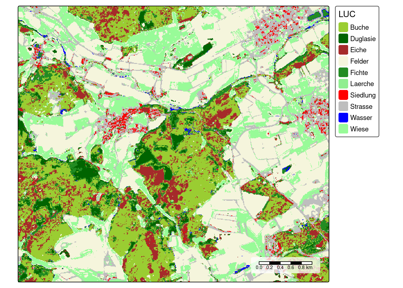
Area of Applicability
We have seen that technically, the trained model can be applied to the entire area of interest (and beyond…as long as the sentinel predictors are available which they are, even globally). But we should assess if we SHOULD apply our model to the entire area. The model should only be applied to locations that feature predictor properties that are comparable to those of the training data. If dissimilarity to the training data is larger than the dissimmilarity within the training data, the model should not be applied to this location.
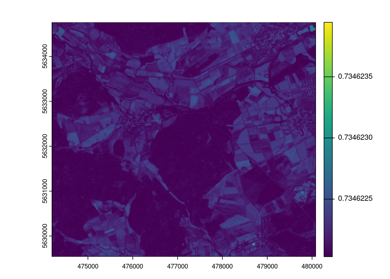
AOA <- aoa(mof_sen,model,LPD=TRUE, verbose=FALSE)
plot(AOA$AOA)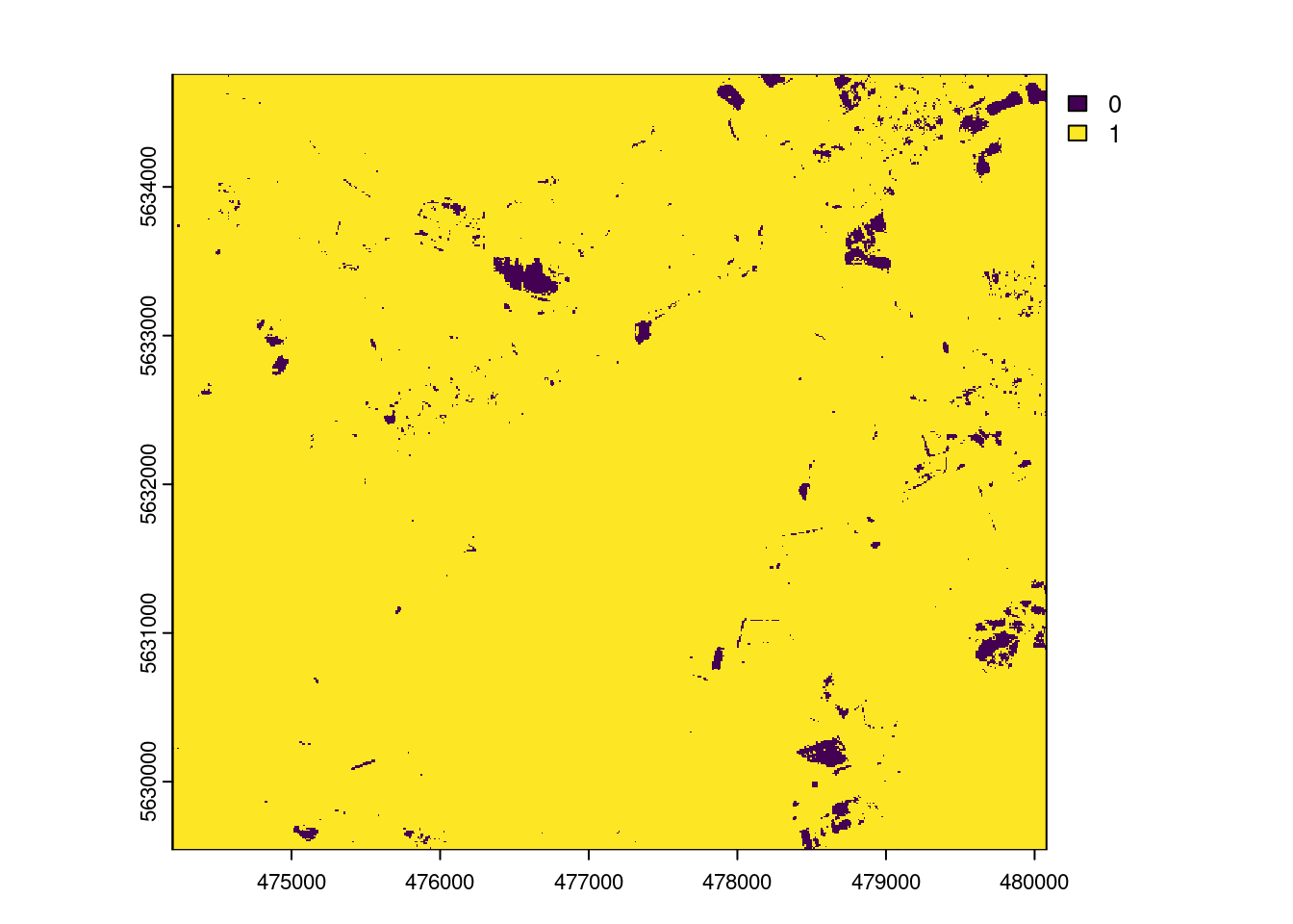
The result of the aoa function has two layers: the dissimilarity index (DI) and the area of applicability (AOA). The DI can take values from 0 to Inf, where 0 means that a location has predictor properties that are identical to properties observed in the training data. With increasing values the dissimilarity increases. The AOA has only two values: 0 and 1. 0 means that a location is outside the area of applicability, 1 means that the model is inside the area of applicability. As an option, we cal also calculate the Local Point Density (LPD), which tells us, for a prediction location, how MANY similar training data points were used during modle training.
Error profiles
Let’s assume there is a relationship between the density of training data points in the predictor space (LPD) and the model performance. Let’s analyze that and use that to predict the prediction performance.
plot(AOA$LPD)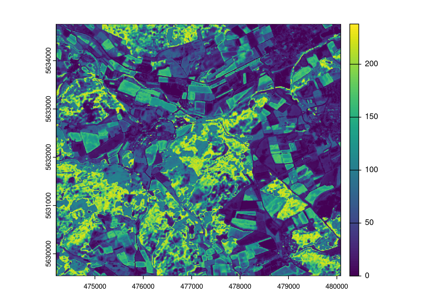
ep <- errorProfiles(model,AOA,variable="LPD")
plot(ep)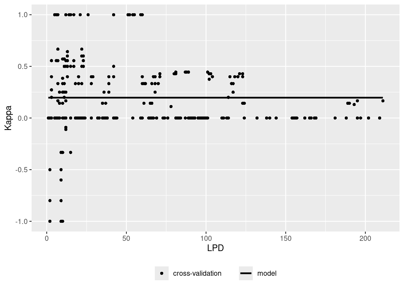
plot(predict(AOA$LPD,ep))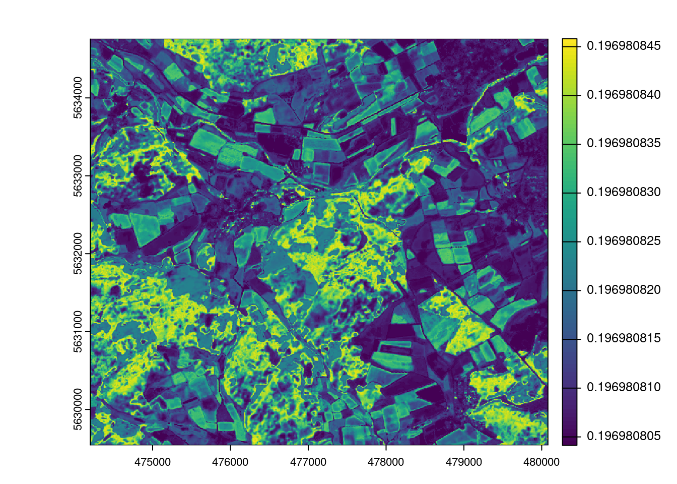
Case Study 2: Modelling the Leaf Area Index
In the second example we will look at a regression task: We have point measurements of Leaf area index (LAI), and, based in this, we would like to make predictions for the entire forest. Again, we will use the Sentinel data as potnetial predictors.
Prepare data
mof_sen <- rast("data/sentinel_uniwald.grd")
LAIdat <- st_read("data/trainingsites_LAI.gpkg")
Reading layer `trainingsites_LAI' from data source
`/home/hanna/Documents/Github/earth-observation-network/EON2025/ml_session/data/trainingsites_LAI.gpkg'
using driver `GPKG'
Simple feature collection with 67 features and 10 fields
Geometry type: POINT
Dimension: XY
Bounding box: xmin: 476350 ymin: 5631537 xmax: 478075 ymax: 5632765
Projected CRS: WGS 84 / UTM zone 32NtrainDat <- extract(mof_sen,LAIdat,na.rm=TRUE)
trainDat$LAI <- LAIdat$LAI
meanmodel <- mof_sen[[1]]
values(meanmodel) <- mean(trainDat$LAI)
plot(meanmodel)
randommodel <- mof_sen[[1]]
values(randommodel)<- runif(ncell(randommodel),min = 0,4)

plot(randommodel)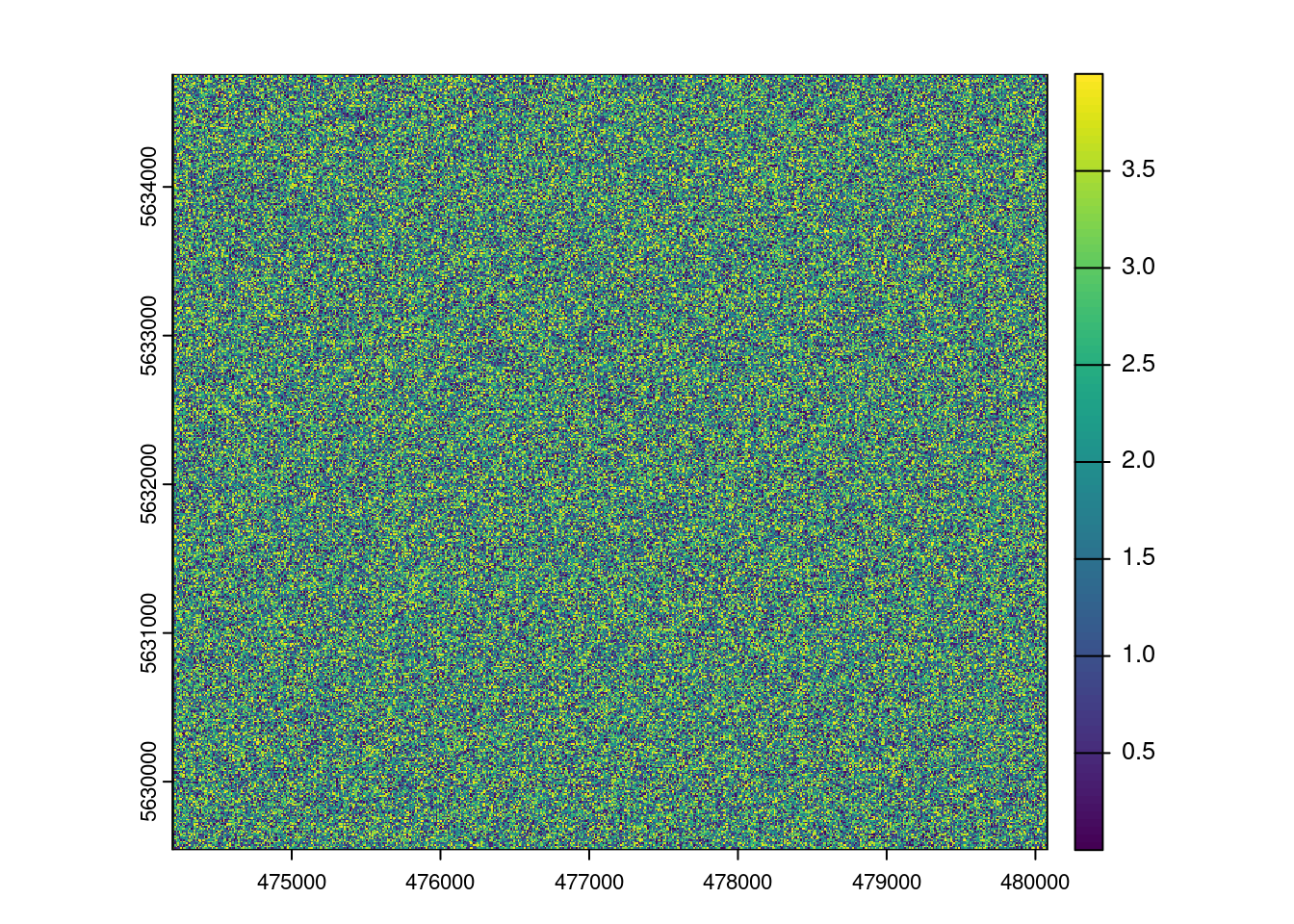
A simple linear model
As a simple first approach we might develop a linear model. Let’s assume a linear relationship between the NDVI and the LAI
plot(trainDat$NDVI,trainDat$LAI)
model_lm <- lm(LAI~NDVI,data=trainDat)
summary(model_lm)
Call:
lm(formula = LAI ~ NDVI, data = trainDat)

Residuals:
     Min       1Q   Median       3Q      Max
-1.87314 -0.52143 -0.03363  0.63668  2.25252

Coefficients:
            Estimate Std. Error t value Pr(>|t|)
(Intercept)  -0.8518     1.4732  -0.578  0.56515
NDVI          6.8433     2.3160   2.955  0.00435 **
---
Signif. codes:  0 '***' 0.001 '**' 0.01 '*' 0.05 '.' 0.1 ' ' 1

Residual standard error: 0.8887 on 65 degrees of freedom
Multiple R-squared:  0.1184,    Adjusted R-squared:  0.1049
F-statistic: 8.731 on 1 and 65 DF, p-value: 0.004354abline(model_lm,col="red")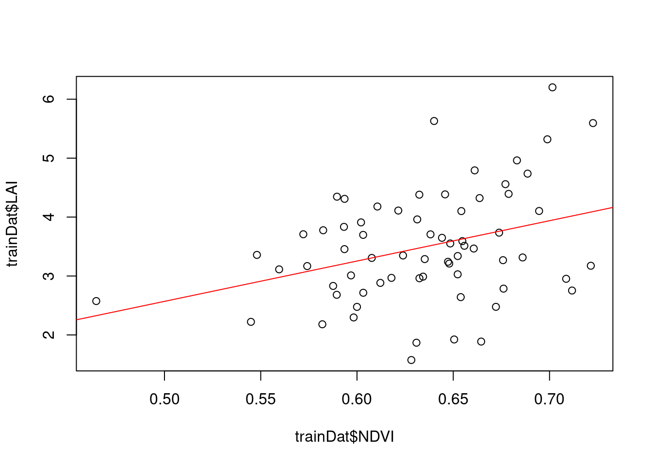
prediction_LAI <- predict(mof_sen,model_lm,na.rm=T)
plot(prediction_LAI)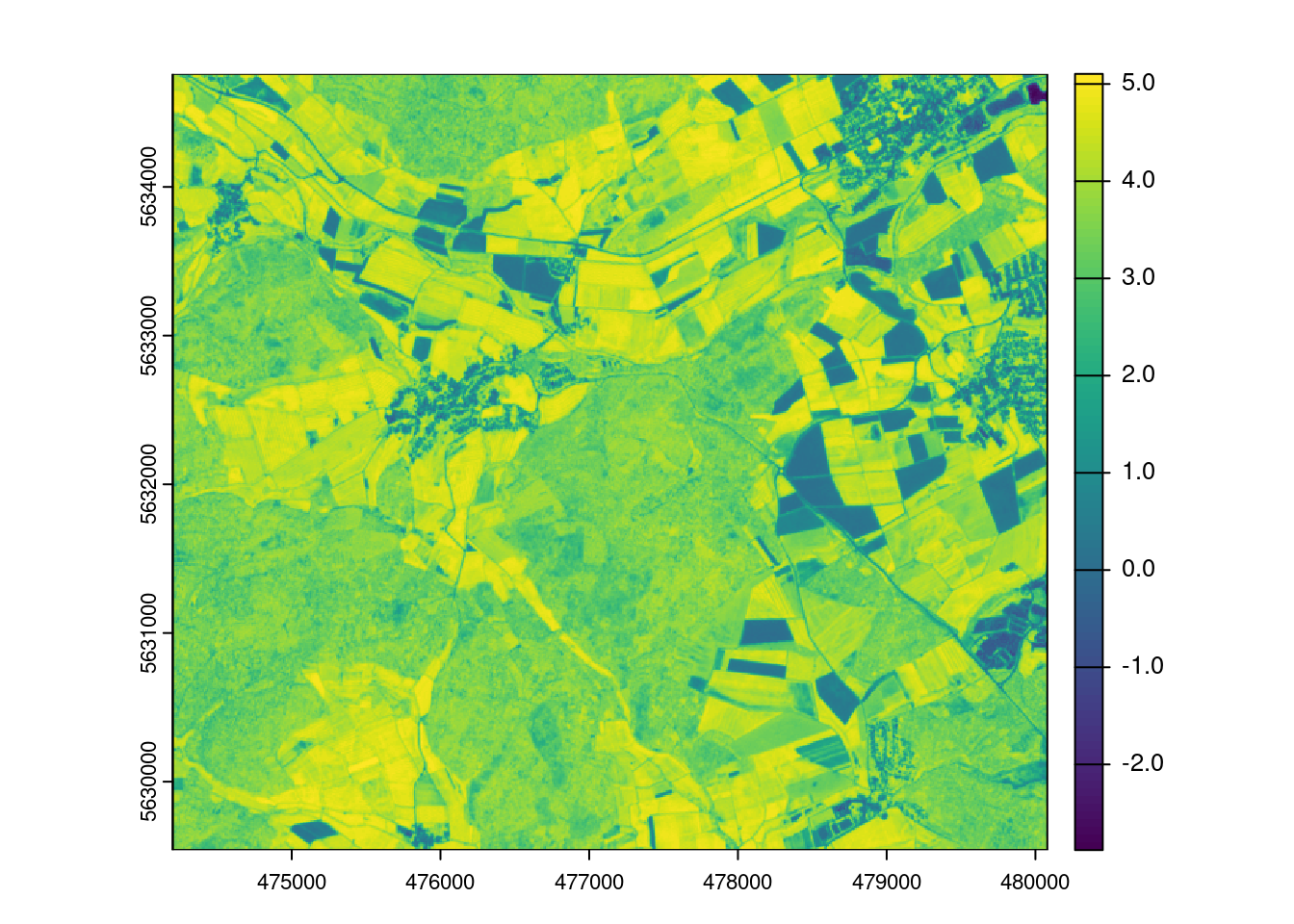
limodelpred <- -0.8518+mof_sen$NDVI*6.8433
mapview(limodelpred)
The machine learning way
Define CV folds
Let’s use the NNDM cross-validation approach.
nndm_folds <- knndm(LAIdat,mof_sen,k=3)Let’s explore the geodistance
gd <- geodist(LAIdat,mof_sen,cvfolds = nndm_folds$indx_test)
plot(gd)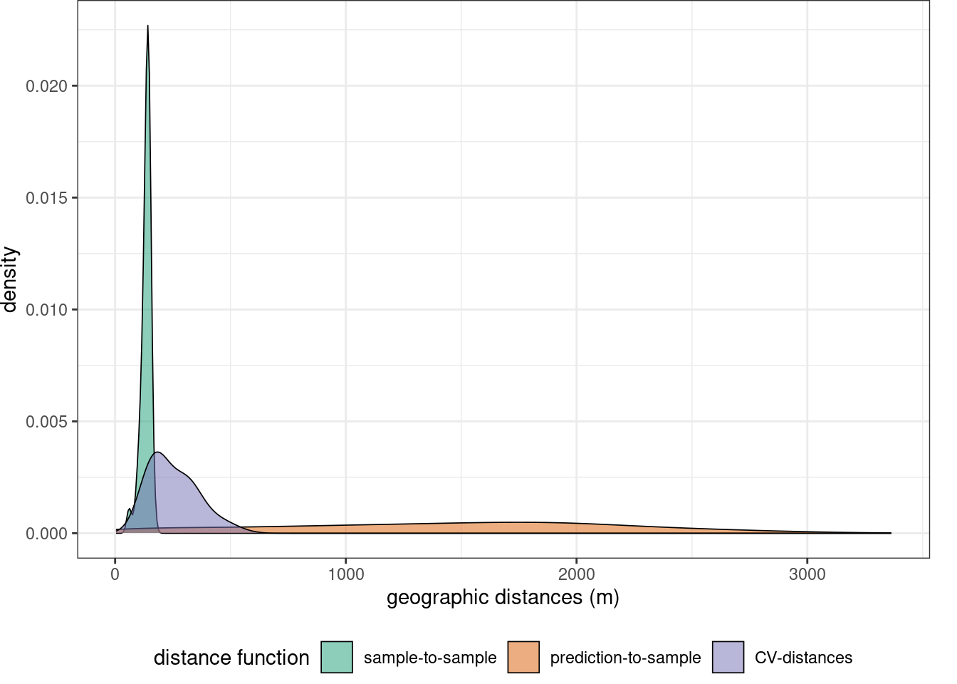
Model training
ctrl <- trainControl(method="cv",
                     index=nndm_folds$indx_train,
                     indexOut = nndm_folds$indx_test,
                    savePredictions = "all")


model <- ffs(trainDat[,predictors],
             trainDat$LAI,
             method="rf",
             trControl = ctrl,
             importance=TRUE,
verbose=FALSE)modelSelected Variables:
T32UMB_20170510T103031_B07 T32UMB_20170510T103031_B08 NDVI
---
Random Forest
67 samples
3 predictor
No pre-processing
Resampling: Cross-Validated (10 fold)
Summary of sample sizes: 41, 44, 49
Resampling results across tuning parameters:
mtry RMSE Rsquared MAE
2 0.8477533 0.2158171 0.7015259
3 0.8612522 0.2068717 0.7236176
RMSE was used to select the optimal model using the smallest value.
The final value used for the model was mtry = 2.LAI prediction
Let’s then use the trained model for prediction.
LAIprediction <- predict(mof_sen,model)
plot(LAIprediction)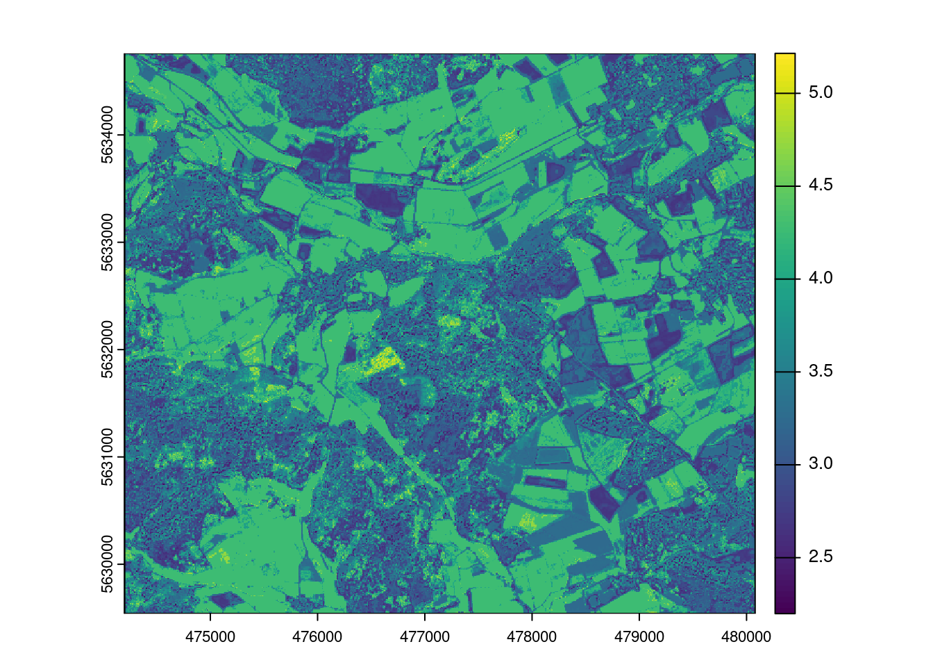
Question?! Why does it look so different than the linear model?
AOA estimation
AOA <- aoa(mof_sen,model,LPD = TRUE, verbose=FALSE)
plot(AOA$AOA)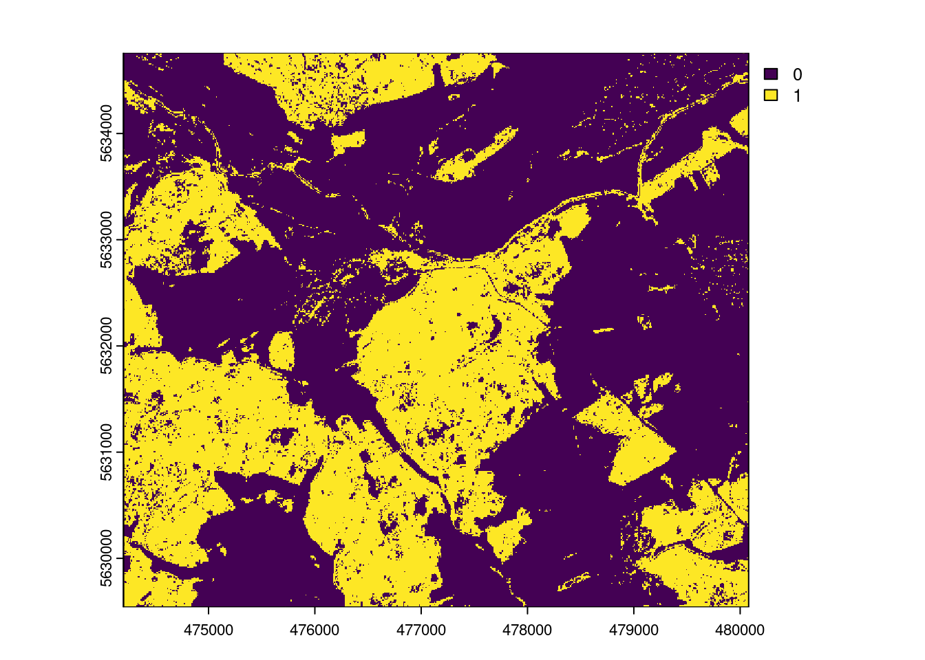
plot(AOA$LPD)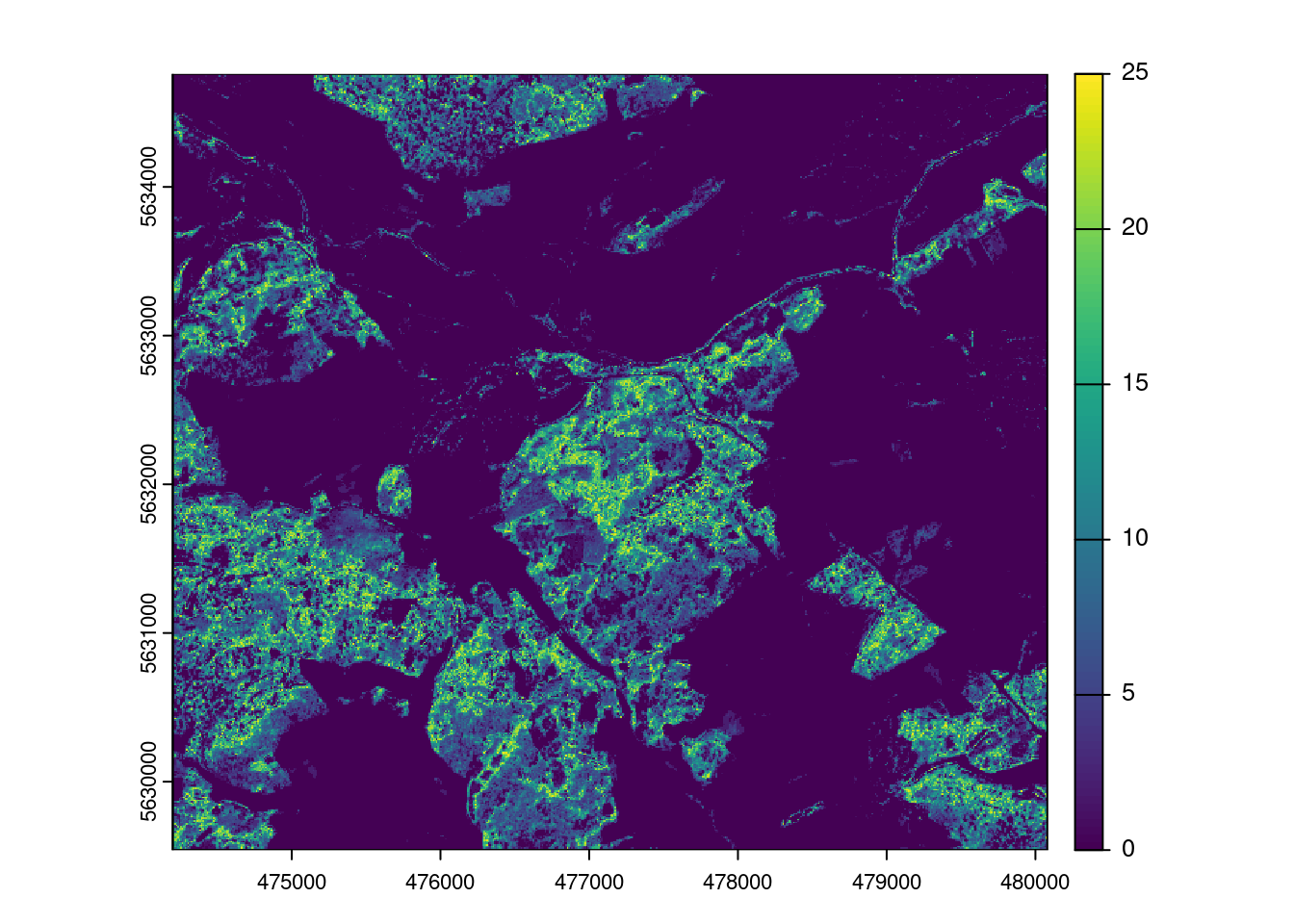
Error profiles
Let’s assume there is a relationship between the density of training data points in the predictor space (LPD) and the model performance. Let’s analyze that and use that to predict the prediction performance.
ep <- errorProfiles(model,AOA,variable="DI")
plot(ep)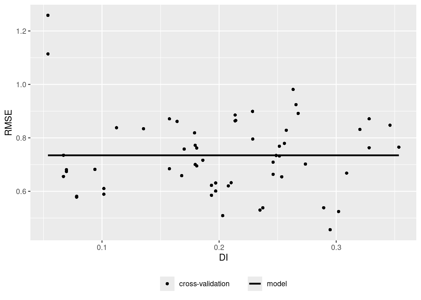
plot(predict(AOA$DI,ep))